Game Math 101, Writing your Own 2D Math in C++

THIS POST IS A WIP

Do you want to make a game but don’t know any math? Do you want to skip endless hours of reading arcane math texts and go straight to the useful stuff? Good! Me too. Let’s just skip straight ahead to the useful stuff. Sit back, grab yourself a lunchable, and get ready to become a wizard.

We will be using C++ and writing our own math to create some demonstrations and animations from scratch. By the end of this article you will produce an interactive experience like the one seen just here below in this cute gif!

gif here

C source code here

This webpage’s source in case you want to post any edits/suggestions/discussion for the article.

Table of Contents

• Prerequisites
• Get a Compiler
• Grab a Copy of tigr
• Build and Run the Math 101 Program
• Drawing some Lines
• Positions (points) and Vectors
• Drawing some Points
• Animating
• Transforming to Screen Space
• Rotations
• Unit Vectors + Normalization
• Dot Product
• Cross Product (aka 2D Determinant)
• Distance and Planes
• Bezier Curves and Lerp
• Matrices
• Transforms
• Raycasting Basics
• Collision Detection Basics
• Toy Demo

Prerequisites

You’ll need to know some basic C++ (well, more like just some basic C stuff), but not much so don’t be worried. If you’re not quite comfortable feel free to visit some online C++ tutorials and then come back here later to try again. At a minimum I’d recommend learning about these topics:

• Loops
• If-statements
• Functions
• Structs

Get a Compiler

Since we’re using C++ we need a compiler. If you already have one and are familiar with how to use them, skip ahead. For those on Mac/Windows here’s how I recommend setting up the g++ compiler.

Make a Folder for this Article

Go ahead and make your own personal folder for holding all the files for this article. I’d recommend naming it math_101.

Windows

If you’re on Windows I recommend to use TDM-GCC, a dead-simple compiler distribution for g++. Just download the installer and open up a command prompt after you install the compiler. Here’s a gif showing how to open a command prompt in a specific window (below). You can also use the cd command to move the command prompt to another folder. Move it to your math_101 folder.

Mac

On Mac just download Xcode from the App Store. This will automatically install the command line tools for you, including g++. Open up the terminal application after you install Xcode. You can also use the cd command to move the terminal to another folder. Move it to your math_101 folder.

Most people reading this article will be using a Windows machine. One Windows they use command prompt instead of Terminal. Later when reading, if you see “command prompt” just think Terminal instead. The rest of the steps are 99% the same, despite this difference.

Linux

If you’re on Linux then I’ll assume you’re already quite familiar with C/C++ and compilers.

Grab a Copy of tigr

We’re using the tigr library. It’s the easiest possible graphics library to get running and use. It handles a bunch of OpenGL stuff for us, in case you were curious. It consists of merely one header file and one source file. Grab a copy of each and put them into your math_101 folder.

• tigr.h
• tigr.c

Build and Run the Math 101 Program

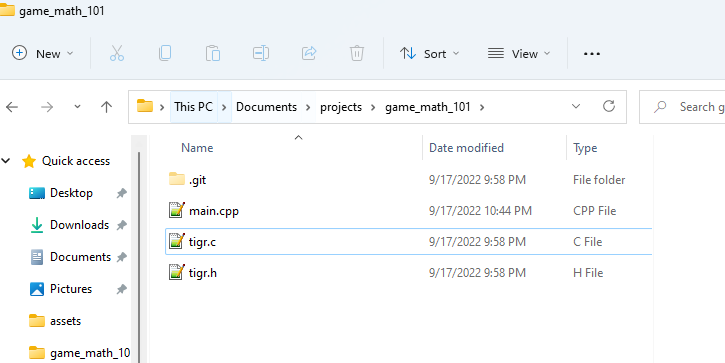
Make a file called main.cpp in your math_101 folder. Copy + paste this code snippet into your main.cpp file.

#include "tigr.h"

int main()
{
	Tigr* screen = tigrWindow(640, 480, "Math 101", 0);

	while (!tigrClosed(screen) && !tigrKeyDown(screen, TK_ESCAPE)) {
		tigrClear(screen, tigrRGB(0x80, 0x90, 0xa0));
		tigrUpdate(screen);
	}

	tigrFree(screen);

	return 0;
}

This code sets up our nice little window to create cool animations and visualize our math as we learn. We must compile this code to create an executable. Make sure your command prompt is opened in the math_101 folder along with tigr.c, tigr.h and main.cpp. It should look something like this (you can ignore the .git file).

Here is the command we will use to compile the code on Windows.

g++ main.cpp tigr.c -o math_101_program -s -lopengl32 -lgdi32

And here is the one for Mac.

g++ main.cpp tigr.c -o math_101_program -framework OpenGL -framework Cocoa

And finally for you Linux weirdos (joking, haha).

g++ main.cpp tigr.c -o math_101_program -s -lGLU -lGL -lX11

If you already know how to use a make and a makefile you can optionally use this makefile. But this is completely optional and not necessary.

ifeq ($(OS),Windows_NT)
	LDFLAGS = -s -lopengl32 -lgdi32
else
	UNAME_S := $(shell uname -s)
	ifeq ($(UNAME_S),Darwin)
		LDFLAGS = -framework OpenGL -framework Cocoa
	else ifeq ($(UNAME_S),Linux)
		LDFLAGS = -s -lGLU -lGL -lX11
	endif
endif

demo : demo.cpp tigr.c
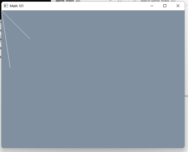
	g++ $^ -Os -o $@ $(CFLAGS) $(LDFLAGS)

This will produce an executable file called math_101_program. Go ahead and run it! You should see a nice ugly window like this one.

Congrats!

Drawing some Lines

The function tigrLine will draw us lines. All we need to do is specify where the line starts, ends, and it’s color. Here’s the function signature from the header file along with the documentation comments found in tigr.h.

// Draws a line.
// Start pixel is drawn, end pixel is not.
// Clips and blends.
void tigrLine(Tigr *bmp, int x0, int y0, int x1, int y1, TPixel color);

x0 and y0 is the first point of the line, while x1 and y are the end point. Add a few calls to tigrLine to our main.cpp program like so:

#include "tigr.h"

int main()
{
	Tigr* screen = tigrWindow(640, 480, "Math 101", 0);

	while (!tigrClosed(screen) && !tigrKeyDown(screen, TK_ESCAPE)) {
		tigrClear(screen, tigrRGB(0x80, 0x90, 0xa0));

        	// Add these two lines here!
		tigrLine(screen, 0, 0, 100, 100, tigrRGB(0xFF, 0xFF, 0xFF));
		tigrLine(screen, 0, 0, 30, 200, tigrRGB(0xFF, 0xFF, 0xFF));

		tigrUpdate(screen);
	}

	tigrFree(screen);

	return 0;
}

It should look like this:

Positions (points) and Vectors

You’ve already used them in the last section on drawing lines! A vector is just a collection of numbers, each number called a component. For games it’s very common to use 2D, 3D, and occassionally 4D vectors. For this article let’s just stick with 2D vectors. Usually we use vectors to represent positions, velocities, and directions. For each of these vectors there would be an x and y a component.

We can write a vector like {x, y}, or (x, y), or even just v. In our program we can use a struct to represent a vector as a pair of two floats.

struct v2
{
    v2() { }
    v2(float x, float y) { this->x = x; this->y = y; }
	float x;
	float y;
};

v2 stands for vector 2, for a 2D vector. We will be writing v2 a lot so it’s best to choose a very short and convenient name. Many other folks like to use vec2 or Vec2, but I’ll recommend a nice a clean v2.

Operations on vectors are what make them useful. The simplest ones are addition and subtraction. We can add two vectors together or subtract two vectors from each other by adding and subtracting their components. By using operator overloading we can easily implement these operations in C++.

v2 operator+(v2 a, v2 b)
{
    return v2(a.x + b.x, a.y + b.y);
}

v2 operator-(v2 a, v2 b)
{
    return v2(a.x - b.x, a.y - b.y);
}

Though from here on out let’s just pack these functions up onto a single line each. We’re going to write a lot of them!

v2 operator+(v2 a, v2 b) { return v2(a.x + b.x, a.y + b.y); }
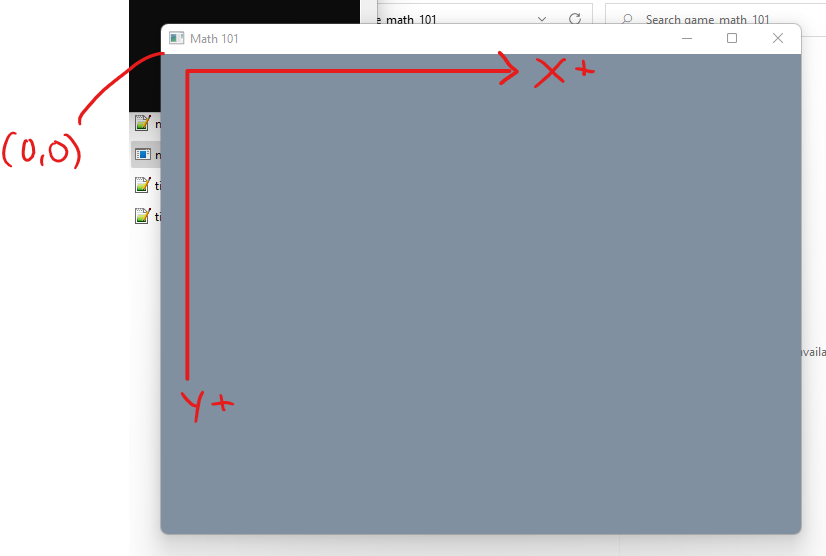
v2 operator-(v2 a, v2 b) { return v2(a.x - b.x, a.y - b.y); }

In our program the coordinate (0, 0) represents the origin of the screen and sits a the top-left. The positive x-axis points to the right, while the positive y-axis points down.

When we drew lines in the last section we actually used vectors. Technically speaking a vector is a direction while a point has a position (or location). (0, 0) is a point at the origin, and (100, 100) is also a point at the end of one of our lines. The difference between these two points is a vector. In this way we can say the vector (a direction) of (100, 100) is used to point at the position (100, 100) from the position (0, 0).

If we wanted to be completely strict about our distinction of points and vectors we could adjust our type definitions and operators. We’re not going to actually do this though, because it’s just not practical. But for learning it’s critical to really nail the difference of points and vectors. Here are a couple quick rules:

1. A position has two components and represents a point in 2D space. We can write it as (x, y), and represent it in code as a v2 float pair. For example, the top-left pixel in our program (the origin) has the position of (0, 0).
2. A position has no orientation or direction. It’s merely a point. An infinitesimally tiny spot.
3. A vector also has two components, and as far as the computer is concerned it looks the same as vector: two floats as a pair, such as (x, y).
4. A vector is a direction, as if it points in a certain direction. For example, so far the direction (0, 1) in our program point straight donwnward.
5. A vector has no position.

So a position has no direction, and a direction has no position. To be somewhere in the world we need a position. To know where something else is in the world, we need not only a position but a direction. Directions are like differences between positions.

When we drew a line in the last section, we could say we drew a vector between two input points (x0, y0) and (x1, y1). However, we could also say we drew a point and vector, or a vector and a point. These are all mathematically equivalent. Let us name a couple variables.

pa = (30, 50)
pb = (200, 350)

We have pa and pb, standing for point A and point B. We can subtract two points to get a vector.

v = pb - ab
-v = pa - pb

In the above example v would have the value of (170, 300). If we do pb - pa this should read like so: the vector between two points is the endpoint minus the start point. Memorize this and burn it into your skull. If we flip the terms around and do pa - pb we get a negative vector (-170, -300). Some more rules pop up!

1. The difference (subtraction) of two points is a vector.
2. The vector between two points is the endpoint minus the start point.

Similarly we can move a points position by addition. We can add a vector to a point and get a new point. Much like how we can subtract a vector from a point and get a new point.

1. A point added with a vector moves the point along the vector.
2. A point subtracted with a vector moves the point along the negative vector.

Drawing some Points

We can draw a single pixel at a specified point with the function tigrPlot. Here’s the signature and docs from the header tigr.h:

// Plots a pixel.
// Clips and blends.
// For high performance, just access bmp->pix directly.
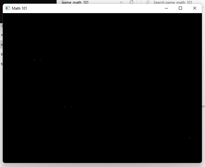
void tigrPlot(Tigr *bmp, int x, int y, TPixel pix);

Let’s use this function to draw a couple pixels. The color of the background is set to black and the points will be white pixels, so we can see them a little easier. tigrPlot takes integers to draw an exact pixel while our v2 struct is floats. We can just typecast the floats to ints to snap each float to specific pixel and draw it as a point.

void draw_point(v2 p, TPixel color)
{
    tigrPlot(screen, (int)p.x, (int)p.y, color);
}

Go ahead and add it to our program, along with our math functions. Let’s also add in some convenience functions to define specific colors for us, like color_white and color_black.

#include "tigr.h"

struct v2
{
	v2() { }
	v2(float x, float y) { this->x = x; this->y = y; }
	float x;
	float y;
};

v2 operator+(v2 a, v2 b) { return v2(a.x + b.x, a.y + b.y); }
v2 operator-(v2 a, v2 b) { return v2(a.x - b.x, a.y - b.y); }

Tigr* screen;

void draw_point(v2 p, TPixel color)
{
    tigrPlot(screen, (int)p.x, (int)p.y, color);
}

TPixel color_white() { return tigrRGB(0xFF, 0xFF, 0xFF); }
TPixel color_black() { return tigrRGB(0, 0, 0); }

int main()
{
	screen = tigrWindow(640, 480, "Math 101", 0);

	while (!tigrClosed(screen) && !tigrKeyDown(screen, TK_ESCAPE)) {
		tigrClear(screen, color_black());
  
        v2 a = v2(200, 300);
        v2 b = v2(100, 150);
        v2 c = v2(600, 400);

		draw_point(a, color_white());
		draw_point(b, color_white());
		draw_point(c, color_white());

		tigrUpdate(screen);
	}

	tigrFree(screen);

	return 0;
}

We can use the above rules to move these points. We can add or subtract a vector. Here’s a program to move all three white points and draw the moved ones as green offset to the right by 20 pixels.

#include "tigr.h"

struct v2
{
	v2() { }
	v2(float x, float y) { this->x = x; this->y = y; }
	float x;
	float y;
};

v2 operator+(v2 a, v2 b) { return v2(a.x + b.x, a.y + b.y); }
v2 operator-(v2 a, v2 b) { return v2(a.x - b.x, a.y - b.y); }

Tigr* screen;

void draw_point(v2 p, TPixel color)
{
	tigrPlot(screen, (int)p.x, (int)p.y, color);
}

TPixel color_white() { return tigrRGB(0xFF, 0xFF, 0xFF); }
TPixel color_black() { return tigrRGB(0, 0, 0); }
TPixel color_red() { return tigrRGB(0xFF, 0, 0); }
TPixel color_green() { return tigrRGB(0, 0xFF, 0); }
TPixel color_blue() { return tigrRGB(0, 0, 0xFF); }

int main()
{
	screen = tigrWindow(640, 480, "Math 101", 0);

	while (!tigrClosed(screen) && !tigrKeyDown(screen, TK_ESCAPE)) {
		tigrClear(screen, color_black());

		v2 a = v2(200, 300);
		v2 b = v2(100, 150);
		v2 c = v2(600, 400);

		draw_point(a, color_white());
		draw_point(b, color_white());
		draw_point(c, color_white());

		// Draw our points moved by the `offset` with green.
		v2 offset = v2(20, 0);

		draw_point(a + offset, color_green());
		draw_point(b + offset, color_green());
		draw_point(c + offset, color_green());

		tigrUpdate(screen);
	}

	tigrFree(screen);

	return 0;
}

Animating

In games we often used what’s called an axis-aligned bounding box (or aabb for short). It means a box that’s aligned onto the x and y axis. We can define an aabb struct in a few ways by using our knowledge of points (positions) and vectors (direction).

// Option 1.
struct aabb
{
    v2 min;
    v2 max;
};

// Option 2.
struct aabb
{
    v2 p;    // position
    float w; // width
    float h; // height
};

// Option 3.
struct aabb
{
    v2 p; // position
    v2 e; // extent vector (width, height)
};

// Option 4.
struct aabb
{
    v2 p;  // position
    v2 he; // half-extent vector (width * 0.5, height * 0.5)
};

Each option is functionally equivalent, but which we choose is largely up to preference. By storing 4 floats we can store the minimum amount of information necessary to represent the entire box. Since an axis aligned bounding box has four corners and a location we only need to know two opposing corners and can calculate the others from that info.

Option 1 stores two opposing corners, the lowest x and lowest y as a pair, and the highest x and highest y as a pair. This is my personal favorite, so let’s go with that. We can also define some useful functions for the aabb:

float width(aabb box) { return box.max.x - box.min.x; }
float height(aabb box) { return box.max.y - box.min.y; }
v2 center(aabb box) { return (box.min + box.max) * 0.5f; }

However, for that last function to work properly we must expand our vector operations. It’s possible to multiply a vector with a scalar. A scalar means a single component number, or a float. Simply multiply with the x component, and then the y component. This adjusts the size, or scale of a vector (also known as magnitude).

v2 operator*(v2 a, float b) { return v2(a.x * b, a.y * b); }

In math notation the length of a vector v is |v|.

• Magnitude is the same as length of a vector v |v|
• Scale is the same as length of a vector v |v|
• These terms are all synonymous

When we multiply a vector v, we are multiplying each component, which in turn scales the length by the same value. We can calculate the length of a vector by utilizing the Pythagorean Theorem a^2 + b^c = c^2, where a, b and c are sides of a right triangle.

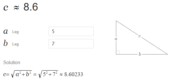
We can think of our vector’s length as c, where a and b are equal to our vectors individual components x and y. We can write down a function to solve for the hypotenuse (or the length of our vector, also known as the magnitude).

#include <math.h> // For sqrtf function.

float length(v2 v)
{
    float a = v.x;
    float b = v.y;
    float c = sqrtf(a * a + b * b);
    return c;
}

Or the shortened version:

float len(v2 v) { return sqrtf(v.x * v.x + v.y * v.y); }

We will make use of this len function later. Now, back to our box drawing function, which will make use of a nifty line drawing function.

void draw_line(v2 a, v2 b, TPixel color)
{
	tigrLine(screen, (int)a.x, (int)a.y, (int)b.x, (int)b.y, color);
}

void draw_box(aabb box, TPixel color)
{
	float w = width(box) + 1;
	float h = height(box) + 1;
	draw_line(box.min, box.min + v2(w, 0), color);
	draw_line(box.min + v2(0,1), box.min + v2(0, h-1), color);
	draw_line(box.max, box.max - v2(w, 0), color);
	draw_line(box.max - v2(0,1), box.max - v2(0, h-1), color);
}

Make a quick mental note that the docs for tigrLine made it clear the last pixel is not drawn, so we add +1 to w/h values to draw one pixel farther.

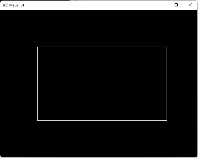
And here’s the program for drawing our box.

#include <math.h>
#include "tigr.h"

struct v2
{
	v2() { }
	v2(float x, float y) { this->x = x; this->y = y; }
	float x;
	float y;
};

v2 operator+(v2 a, v2 b) { return v2(a.x + b.x, a.y + b.y); }
v2 operator-(v2 a, v2 b) { return v2(a.x - b.x, a.y - b.y); }
v2 operator*(v2 a, float b) { return v2(a.x * b, a.y * b); }
float len(v2 v) { return sqrtf(v.x * v.x + v.y * v.y); }

struct aabb
{
	aabb() { }
	aabb(v2 min, v2 max) { this->min = min; this->max = max; }
	v2 min;
	v2 max;
};

float width(aabb box) { return box.max.x - box.min.x; }
float height(aabb box) { return box.max.y - box.min.y; }
v2 center(aabb box) { return (box.min + box.max) * 0.5f; }

Tigr* screen;

void draw_point(v2 p, TPixel color) { tigrPlot(screen, (int)p.x, (int)p.y, color); }
void draw_line(v2 a, v2 b, TPixel color) { tigrLine(screen, (int)a.x, (int)a.y, (int)b.x, (int)b.y, color); }

void draw_box(aabb box, TPixel color)
{
	float w = width(box) + 1;
	float h = height(box) + 1;
	draw_line(box.min, box.min + v2(w, 0), color);
	draw_line(box.min, box.min + v2(0, h), color);
	draw_line(box.max, box.max - v2(w, 0), color);
	draw_line(box.max, box.max - v2(0, h), color);
}

TPixel color_white() { return tigrRGB(0xFF, 0xFF, 0xFF); }
TPixel color_black() { return tigrRGB(0, 0, 0); }
TPixel color_red() { return tigrRGB(0xFF, 0, 0); }
TPixel color_green() { return tigrRGB(0, 0xFF, 0); }
TPixel color_blue() { return tigrRGB(0, 0, 0xFF); }

int main()
{
	screen = tigrWindow(640, 480, "Math 101", 0);

	while (!tigrClosed(screen) && !tigrKeyDown(screen, TK_ESCAPE)) {
		tigrClear(screen, color_black());

		aabb box = aabb(v2(120, 120), v2(540, 360));
		draw_box(box, color_white());

		tigrUpdate(screen);
	}

	tigrFree(screen);

	return 0;
}

And finally let’s animate this box a bit. It’s time to introduce, time… Haha. I’m practicing my dad jokes. tigrTime is a nice function that returns the number of seconds since it was last called as a float. We can use it to calculate a dt variable once per game loop, standing for delta time. This will be used a whole lot later in this article for animating things and calculating movements.

For now we can use time and pass it into cosine and sine functions cosf and sinf from the math.h C runtime header. Go ahead and check out these edits to our program. I added // New code! comments on all the edited lines since the last version.

#include <math.h>
#include "tigr.h"

struct v2
{
	v2() { }
	v2(float x, float y) { this->x = x; this->y = y; }
	float x;
	float y;
};

v2 operator+(v2 a, v2 b) { return v2(a.x + b.x, a.y + b.y); }
v2 operator-(v2 a, v2 b) { return v2(a.x - b.x, a.y - b.y); }
v2 operator*(v2 a, float b) { return v2(a.x * b, a.y * b); }
float len(v2 v) { return sqrtf(v.x * v.x + v.y * v.y); }

struct aabb
{
	aabb() { }
	aabb(v2 min, v2 max) { this->min = min; this->max = max; }
	v2 min;
	v2 max;
};

float width(aabb box) { return box.max.x - box.min.x; }
float height(aabb box) { return box.max.y - box.min.y; }
v2 center(aabb box) { return (box.min + box.max) * 0.5f; }

Tigr* screen;

void draw_point(v2 p, TPixel color) { tigrPlot(screen, (int)p.x, (int)p.y, color); }
void draw_line(v2 a, v2 b, TPixel color) { tigrLine(screen, (int)a.x, (int)a.y, (int)b.x, (int)b.y, color); }

void draw_box(aabb box, TPixel color)
{
	float w = width(box) + 1;
	float h = height(box) + 1;
	draw_line(box.min, box.min + v2(w, 0), color);
	draw_line(box.min, box.min + v2(0, h), color);
	draw_line(box.max, box.max - v2(w, 0), color);
	draw_line(box.max, box.max - v2(0, h), color);
}

TPixel color_white() { return tigrRGB(0xFF, 0xFF, 0xFF); }
TPixel color_black() { return tigrRGB(0, 0, 0); }
TPixel color_red() { return tigrRGB(0xFF, 0, 0); }
TPixel color_green() { return tigrRGB(0, 0xFF, 0); }
TPixel color_blue() { return tigrRGB(0, 0, 0xFF); }

int main()
{
	screen = tigrWindow(640, 480, "Math 101", 0);

	float t = 0; // New code!
	while (!tigrClosed(screen) && !tigrKeyDown(screen, TK_ESCAPE)) {
		float dt = tigrTime(); // New code!
		t += dt; // New code!
		tigrClear(screen, color_black());

		aabb box = aabb(v2(120, 120), v2(540, 360));
		v2 offset = v2(cosf(t), sinf(t)) * 100.0f; // New code!
		box.min = box.min - offset; // New code!
		box.max = box.max + offset; // New code!
		draw_box(box, color_white());

		tigrUpdate(screen);
	}

	tigrFree(screen);

	return 0;
}

Transforming to Screen Space

When we’re talking about games and math the word transform means to go from one coordinate space to another. You’re likely already familiar with the traditional 2D cartesian space, whether or not you’re familiar with the terminology. There are two axes, one for x and one for y. However, it’s possible to take that 2D space and transform it to another space.

The types of transformation we will cover later include:

• Translation
• Scaling (also includes flipping/mirroring)
• Rotating

For now we’ll just cover some translating and flipping. In the math_101 program our coordinate space has the origin at the top-left pixel with the y-axis pointing downward. Though, most games use a different coordinate space for the screen where the origin is at the center, and the y-axis is pointing upwards. We want to use math to transform the screen to this new form.

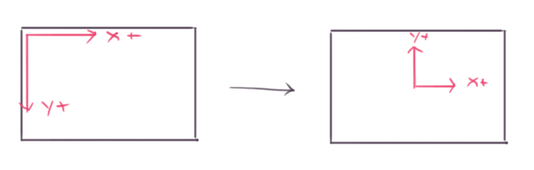
To perform this transformation we can start by negating the y-axis. This will make the y-axis point upwards. We can start writing a function called world_to_screen, which will take a point in our game world with the origin at center of the screen, to the screen coordinates we’ve been using so far.

v2 world_to_screen(v2 p)
{
	p.y = -p.y;
	return p;
}

The next step would be to offset the point by half the screen width and half the screen height, placing points that were originally at (0, 0) at (screen_width / 2, screen_height / 2).

v2 world_to_screen(v2 p)
{
	p.y = -p.y;
	float half_screen_width = 640.0f / 2.0f;
	float half_screen_height = 480.0f / 2.0f;
	p.x += half_screen_width;
	p.y += half_screen_height;
	return p;
}

Now we can hook this function into all of our drawing functions so far. If it works, we should be able to draw a box centered at (0, 0) and have it appear in the center of the screen. It’s also a convenient time to implement operators for +=, -=, *=, and division operators / and /=.

v2 operator+(v2 a, v2 b) { return v2(a.x + b.x, a.y + b.y); }
v2 operator+=(v2& a, v2 b) { a = v2(a.x + b.x, a.y + b.y); return a; }
v2 operator-(v2 a, v2 b) { return v2(a.x - b.x, a.y - b.y); }
v2 operator-=(v2& a, v2 b) { a = v2(a.x - b.x, a.y - b.y); return a; }
v2 operator*(v2 a, float b) { return v2(a.x * b, a.y * b); }
v2 operator*=(v2& a, float b) { a = v2(a.x * b, a.y * b); return a; }
v2 operator/(v2 a, float b) { return v2(a.x / b, a.y / b); }
v2 operator/=(v2& a, float b) { a = v2(a.x / b, a.y / b); return a; }

Our code is getting a bit big, so for now let’s bundle things up into a header called math_101.h. We can place all of our math struct types like v2, aabb, and any other that come along later. Here is our current version of math_101.h.

struct v2
{
	v2() { }
	v2(float x, float y) { this->x = x; this->y = y; }
	float x;
	float y;
};

v2 operator+(v2 a, v2 b) { return v2(a.x + b.x, a.y + b.y); }
v2 operator+=(v2& a, v2 b) { a = v2(a.x + b.x, a.y + b.y); return a; }
v2 operator-(v2 a, v2 b) { return v2(a.x - b.x, a.y - b.y); }
v2 operator-=(v2& a, v2 b) { a = v2(a.x - b.x, a.y - b.y); return a; }
v2 operator*(v2 a, float b) { return v2(a.x * b, a.y * b); }
v2 operator*=(v2& a, float b) { a = v2(a.x * b, a.y * b); return a; }
v2 operator/(v2 a, float b) { return v2(a.x / b, a.y / b); }
v2 operator/=(v2& a, float b) { a = v2(a.x / b, a.y / b); return a; }
float len(v2 v) { return sqrtf(v.x * v.x + v.y * v.y); }

struct aabb
{
	aabb() { }
	aabb(v2 min, v2 max) { this->min = min; this->max = max; }
	v2 min;
	v2 max;
};

float width(aabb box) { return box.max.x - box.min.x; }
float height(aabb box) { return box.max.y - box.min.y; }
v2 center(aabb box) { return (box.min + box.max) * 0.5f; }

The drawing functions can be placed into a header file called draw.h that looks like this:

Tigr* screen;

v2 world_to_screen(v2 p)
{
	p.y = -p.y;
	float half_screen_width = 640.0f / 2.0f;
	float half_screen_height = 480.0f / 2.0f;
	p.x += half_screen_width;
	p.y += half_screen_height;
	return p;
}

void draw_point(v2 p, TPixel color)
{
	p = world_to_screen(p);
	tigrPlot(screen, (int)p.x, (int)p.y, color);
}

void draw_line(v2 a, v2 b, TPixel color)
{
	a = world_to_screen(a);
	b = world_to_screen(b);
	tigrLine(screen, (int)a.x, (int)a.y, (int)b.x, (int)b.y, color);
}

void draw_box(aabb box, TPixel color)
{
	float w = width(box) + 1;
	float h = height(box) + 1;
	draw_line(box.min, box.min + v2(w, 0), color);
	draw_line(box.min, box.min + v2(0, h), color);
	draw_line(box.max, box.max - v2(w, 0), color);
	draw_line(box.max, box.max - v2(0, h), color);
}

TPixel color_white() { return tigrRGB(0xFF, 0xFF, 0xFF); }
TPixel color_black() { return tigrRGB(0, 0, 0); }
TPixel color_red() { return tigrRGB(0xFF, 0, 0); }
TPixel color_green() { return tigrRGB(0, 0xFF, 0); }
TPixel color_blue() { return tigrRGB(0, 0, 0xFF); }

And our current main.cpp program looks like this:

#include <math.h>
#include "tigr.h"
#include "math_101.h"
#include "draw.h"

int main()
{
	screen = tigrWindow(640, 480, "Math 101", 0);

	aabb red_box = aabb(v2(-50, -50), v2(50, 50));
	aabb blue_box = aabb(v2(-50, -50), v2(50, 50));
	while (!tigrClosed(screen) && !tigrKeyDown(screen, TK_ESCAPE)) {
		float dt = tigrTime();
		tigrClear(screen, color_black());

		red_box.min += v2(30.0f, 0) * dt;
		red_box.max += v2(30.0f, 0) * dt;
		blue_box.min += v2(0, 30.0f) * dt;
		blue_box.max += v2(0, 30.0f) * dt;
		draw_box(red_box, color_red());
		draw_box(blue_box, color_blue());

		tigrUpdate(screen);
	}

	tigrFree(screen);

	return 0;
}

When run it will show a red box traveling along our new x-axis starting at the origin, and a blue box traveling along the new y-axis at our new origin.

From here on when we write new math code you can follow along and place it into the math_101.h header! Drawing related functions can go into draw.h. The red box is traveling at 30 pixels per second. We can see this from the expression v2(30.0f, 0) * dt. Whenever we multiply something by dt, it can be read like “over one second”. In this case it’s 30 pixels per second.

NOTE: Those more familiar with C might notice no include guards were used. Don’t worry about this for now; it’s more important to just focus on the math and pump out more code. Our program is just one-file conceptually, and we’re only splitting it up into different files to make following this article easier. TODO - Link to GitHub repo of final demo.

Rotations

Rotations are actually much more easy to perform than they are to learn about. Here comes another one of those rules to burn into your mind: rotations are always done about the origin. This is the truth. Here is how we rotate a vector or point about the origin given an angle in radians.

v2 rotate(v2 v, float radians)
{
	float s = sinf(radians);
	float c = cosf(radians);
	return v2(c * v.x - s * v.y, s * v.x + c * v.y);
}

The first step to understanding rotations is to understand sin and cos functions. For a quick refresher I recommend this page over at mathisfun on the unit circle.

For any vector on the unit circle its length is 1. We can calculate the x and y components of this unit vector with the sin and cos function by providing the angle in radians.

v2 vector_on_unit_circle_from_angle(float radians)
{
	return v2(cosf(radians), sinf(radians));
}

We can think of this as rotating the x-axis (1, 0) by an angle (remember, when writing code cosf and sinf functions work in radians mode). Similarly, we can think about how to rotate the y-axis by the same angle, and we would get a similar result of (-sin(radians), cos(radians)). One way to realize this is from a useful function called skew.

v2 skew(v2 a) { return v2(-a.y, a.x); }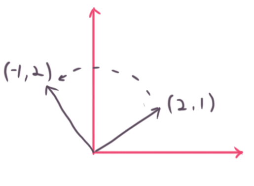

It returns vector rotated by 90 degrees counter-clockwise. To rotate a vector 90 degrees counter-clockwise we flip the x and y components, and negate the x final component. It comes from the concept of a skew-symmetric matrix, one that can perform a cross-product. Other names include pseudo-cross product, or perp-dot product (standing for perpendicular). We won’t really go over these, I’m just mentioning them for anyone curious what the names mean.

As it turns out, whenever we write down any vector, a such as (1, 2) or (10, -13) we are using what’s called a basis, or a space. Our vectors are not merely (1, 2) or (10, -13), they are actually expressed as multipliers of the x and y axes.

(1, 2) and (10, -13) aren’t special vectors or anything, I just chose them as random examples.

10 * x-axis + -13 * y-axis

Thinking about how the x-axis is (1, 0) and the y-axis is (0, 1) we can substitute in these values (which are just 1).

10 * (1, 0) + -13 * (0, 1)
=  (10 * 1, -13 * 1)
=  (10, -13)

And that gets us back to where we started.

Seems pretty silly, right? All that extra work for nothing! Well, when we think about rotations we’re actually rotating the entire coordinate system. The coordinate system (the cartesian grid we talked about earlier) is defined by the x-axis and the y-axis, so we’re actually rotating these two axes when we do a rotation.

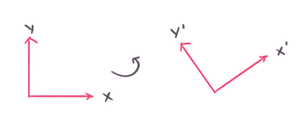
Let’s use the terms i and j for representing a number relative to a basis. Taking our example vector of (10, -13) we can write it down as it would be shown in left-hand diagram as 10 * i + -13 * j. So what would i and j be for the rotated basis (x’, 0) + (0, y’) by an angle a? From our understanding of the unit circle the x-axis would be (cos(a), sin(a)). We can use this for our i vector. To get the j vector we rotate the x-axis by 90 degrees counter-clockwise using our skew function and get (-sin(a), cos(a)). To represent (10, -13) relative to our new i and j vectors we just use the formula from earlier.

10 * i + -13 * j
i = (cos(a), sin(a))
j = (-sin(a), cos(a))

substitute in =>

10 * (cos(a), sin(a))
-13 * (-sin(a), cos(a)))

And there we have it! Rotating a vector by an angle is the same as expressing the vector in a rotated coordinate frame (or basis). We can rotate any vector by changing 10 and -13 to x and y input variables to arrive back at our original function.

v2 rotate(v2 v, float a)
{
	float s = sinf(a);
	float c = cosf(a);
	return v2(c * v.x - s * v.y, s * v.x + c * v.y);
}

If this was all over your head don’t sweat it. You can just use the rotate function as a black-box without understanding the internals and that’s a totally valid way to make games. As long as you memorize the rules you’ll be good to go, such as the rule we mentioned at the beginning of this section: rotations are always performed about the origin.

But what if we want to rotate around some other point? For example say we want to create a special effect where a ball of light is circling around an enemy somewhere on the screen other than the origin? It turns out there’s a very simple solution. Just translate the enemy’s location to the origin, apply the rotation, then translate back.

v2 rotate_point_a_around_point_b(v2 a, v2 b, float radians)
{
	// Compute cosine and sine values for our i and j vectors.
	float c = cosf(radians);
	float s = sinf(radians);

	// Translate so that b is the origin.
	a = a - b; 

	// Rotate a around the origin.
	// a' = a.x * i + a.y * j
	// where i = (c, s), j = (-s, c)
	// substitute =>
	// a' = a.x * (c, s) + a.y * (-s, c)
	a = v2(c * a.x - s * a.y, s * a.x + c * a.y);

	// Translate back to b.
	return a + b;
}

The functions cosf and sinf are quite fast on modern processors, but still should be thought of as an order of magnitude (10x) slower than a normal float multiply. Therefore it’s going to be preferable to precompute these values whenever we can and store them. A good way for our math library to make use of rotations is to make a struct representing a rotation. It can be multiplied with vectors to rotate them by an angle.

struct rotation
{
	float s;
	float c;
};

rotation sincos(float a) { rotation r; r.c = cosf(a); r.s = sinf(a); return r; }
v2 mul(rotation a, v2 b) { return v2(a.c * b.x - a.s * b.y, a.s * b.x + a.c * b.y); }

We can build a rotation by calling sincos, and then rotate a vector with it by calling mul. Alternatively you could implement an operator* to perform rotations, however I recommend using a mul function for a few reasons.

• mul can be easily overloaded without modifying the “class definition”. Just simply add more mul functions later on for different kinds of operations.
• Post-multiplication or pre-multiplication (e.g. 5 * x vs x * 5) can be expressed in a more explicit manner. For example if we write a * b * c, what is the order of operations supposed to be? Of course the C/C++ programming languages clearly define the order of operations, but if we’re writing down hand-written math notes and want to transcribe it into code, it’s in my opinion more clear what the intent is if we write down mul(a, mul(b, c)) or mul(mul(a, b), c). This distinction matters a lot later down the line when we are dealing with transforms and matrices, where multiplication is non-commutative.

It’s time to throw our rotation functions into practice and generate a bunch lines rotated around the origin like the spokes of a bicycle wheel.

#include <math.h>
#include "tigr.h"
#include "math_101.h"
#include "draw.h"

int main()
{
	screen = tigrWindow(640, 480, "Math 101", 0);

	float t = 0;
	while (!tigrClosed(screen) && !tigrKeyDown(screen, TK_ESCAPE)) {
		float dt = tigrTime();
		t += dt;
		tigrClear(screen, color_black());

		v2 p = v2(100.0f, 0);
		rotation r = sincos(t * 0.01f);
		for (int i = 0; i < 32; ++i) {
			draw_line(v2(0, 0), p, color_white());
			p = mul(r, p);
		}

		tigrUpdate(screen);
	}

	tigrFree(screen);

	return 0;
}

Unit Vectors + Normalization

You must have this super useful vector drawing function in your rendering arsenal. Used to visualize vectors at a specific location (remember, a vector is merely a direction, as drawing a vector must happen at a location), the vector drawing function can save us from many headaches down the line whenever we must debug our code and figure out what’s going on.

By taking an input vector and position we can draw an arrow shape on the screen. The arrowhead will show us which way the vector is facing. We can provide a scale factor to the function to adjust the size of the arrowhead. The way it works is we calculate by-hand the arrow’s position when it’s sitting along the x-axis. Using our newfound knowledge on rotations we can then rotate all of the points that define the arrow about the origin, and then translate them to the position as a final step. Remember, rotations always happen about the origin. If we translate first then rotate the results will be wrong. I encourage you to try this out as an experiment and see what it looks like!

We need some help from a helpful function called atan2, the function used to compute the angle from the x-axis to a vector.

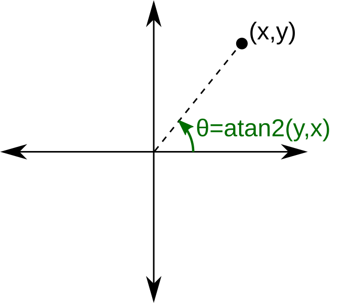
Since atan2 returns a number from pi to -pi it’s often helpful to remap this from 0 to 2 * pi by adding pi to the result of atan2. Let’s implement a few overloads for our own atan2_360 function, which returns a value from 0 to 2 * pi (or 360 degrees). It’s definitely appropriate to black-box the atan2 function and not worry too much about how it works.

float atan2_360(float y, float x) { return atan2f(-y, -x) + 3.14159265f; }
float atan2_360(rotation r) { return atan2_360(r.s, r.c); }
float atan2_360(v2 v) { return atan2f(-v.y, -v.x) + 3.14159265f; }

void draw_vector(v2 p, v2 v, TPixel color)
{
	v2 arrow[] = {
		v2(0.0f, 0.0f),
		v2(-5.0f, 5.0f),
		v2(0.0f, 0.0f),
		v2(-5.0f, -5.0f),
	};
	rotation r = sincos(atan2_360(v));
	for (int i = 0; i < 4; ++i) {
		arrow[i] = mul(r, arrow[i]);
		arrow[i] += p + v;
	}
	draw_line(arrow[0], arrow[1], color);
	draw_line(arrow[2], arrow[3], color);
	draw_line(p, p + v, color);
}

However, we can optimize the draw_vector function by not using atan2 at all. We can calculate the rotation directly with a little bit of math. Using the knowledge from the previous section about rotations we can just write down the formula for sin and cos values needed to rotate the x-axis to an any vector without calling into cosf, sinf or atan2f.

Recall from the previous section on rotations for how to rotate the x-axis by an angle.

x = (1, 0) // The x-axis.
a = angle
x' = (1 * cos(a) - 0 * sin(a), 1 * sin(a) + 0 * cos(a))

We already know x’, it’s the v vector we want to draw. We can see that v.x = cos(a) and v.y = sin(a). Since we already know sin(a) and cos(a) we can skip atan2 and directly create a rotation. However, our function draw_vector works with non-unit vectors v. We can deal with non-unit vectors (vectors whose lengths are not 1) by normalizing the v. Normalization is the process of computing a vector’s length then dividing the vector by the length. This returns a unit vector pointing in the direction the original vector was pointing. Let’s call it norm for shorthand.

v2 norm(v2 v) { float l = len(v); return v * (1.0f / l); }

We can normalize v before grabbing it’s x and y components and treating them as sin/cos values.

// In math_101.h ...
struct rotation
{
	// Add some constructors here.
	rotation() { }
	rotation(float angle) { s = sinf(angle); c = sinf(angle); }
	rotation(float s, float c) { this->s = s; this->c = c; }
	float s;
	float c;
};

// In draw.h ...
void draw_vector(v2 p, v2 v, TPixel color)
{
	v2 arrow[] = {
		v2(0.0f, 0.0f),
		v2(-5.0f, 5.0f),
		v2(0.0f, 0.0f),
		v2(-5.0f, -5.0f),
	};
	v2 n = norm(v);
	rotation r = rotation(n.y, n.x);
	for (int i = 0; i < 4; ++i) {
		arrow[i] = mul(r, arrow[i]);
		arrow[i] += p + v;
	}
	draw_line(arrow[0], arrow[1], color);
	draw_line(arrow[2], arrow[3], color);
	draw_line(p, p + v, color);
}

Congratulations! You just optimized away atan2f, sinf and cosf calls and replaced them with a single sqrtf call (inside of our len and norm functions)!

The final thing we can change is adding in a scale value. Recall from earlier that scaling a vector is merely multiplying it’s components by the scale factor. Sear this rule into your brain: scaling happens about the origin. Period. If you wish to scale about another point simply translate to the origin first, then translate back after.

void draw_vector(v2 p, v2 v, TPixel color, float scale = 5.0f)
{
	v2 arrow[] = {
		v2(0.0f, 0.0f),
		v2(-1.0f, 1.0f),
		v2(0.0f, 0.0f),
		v2(-1.0f, -1.0f),
	};
	v2 n = norm(v);
	rotation r = rotation(n.y, n.x);
	for (int i = 0; i < 4; ++i) {
		arrow[i] *= scale;           // Scale first (about the origin).
		arrow[i] = mul(r, arrow[i]); // Then rotate (about the origin).
		arrow[i] += p + v;           // And finally translate.
	}
	draw_line(arrow[0], arrow[1], color);
	draw_line(arrow[2], arrow[3], color);
	draw_line(p, p + v, color);
}

This function scales the arrowhead about the origin, then rotate’s about the origin, and finally translates.

Dot Product

If you were asked what the most critical math function in call of gamedev is, what might the answer be? It better darned be the dot product! The core math function used in almost every geometric calculation ever, it’s used to calculate some information about how two vectors relate to each other. It can be used to understand the angle between vectors, wether vectors are facing each other or not, and as an optimized was to compute the cos of the angle between two vectors without actually calling the cosf function.

The dot product comes from the law of cosines. Here’s the formula:

Equation 1

c^2 = a^2 + b^2 – 2ab * cos(γ)

This is just an equation that relates the cosine of an angle within a triangle to its various side lengths a, b and c. The Wikipedia page on the law of cosines (link above) does a nice job of explaining this in excrutiating detail. Equation 1 can be rewritten as:

Equation 2

c^2 – a^2 – b^2 = -2ab * cos(γ)

The right hand side equation Equation 2 is interesting! Lets say that instead of writing the equation with side lengths a, b and c, it is written with two vectors: u and v. The third side can be represented as u – v. Recall that |v| means the length of v, computed by using the Pythagorean Thereom. Re-writing equation Equation 2 in vector notation yields:

Equation 3

|u - v|^2 – |u|^2 – |v|^2 = -2|u||v| * cos(γ)

Which can be expressed in scalar form as:

Equation 4

(u.x - v.x)^2 + (u.y - v.y)^2 + (u.z - v.z)^2 -
((u.x)^2 + (u.y)^2 + (u.z)^2) - ((v.x)^2 + (v.y)^2 + (v.z)^2) =
-2|u||v| * cos(γ)

By crossing out some redundant terms, and getting rid of the -2 on each side of the equation, this ugly equation can be turned into a much more approachable version:

Equation 5

u.x * v.x + u.y * v.y + u.z * v.z = |u||v| * cos(γ)

Equation 5 is the equation for the dot product. If both u and v are unit vectors then the equation will simplify to:

Equation 6

dot(u, v) = cos(γ)

If u and v are not unit vectors equation 5 says that the dot product between both vectors is equal to cos(γ) that has been scaled by the lengths of u and v. This is a nice thing to know! For example: the squared length of a vector is just itself dotted with itself. We can use this knowledge to rewrite our len function with the dot product.

float len(v2 v) { return sqrtf(v.x * v.x + v.y * v.y); }
// =>
float dot(v2 a, v2 b) { return a.x * b.x + a.y * b.y; }
float len(v2 v) { return sqrtf(dot(v, v)); }

If u is a unit vector and v is not, then dot(u, v) will return the distance in which v travels in the u direction. We will make prolific use of the dot product later! Here are the footnotes of some useful dot product properties:

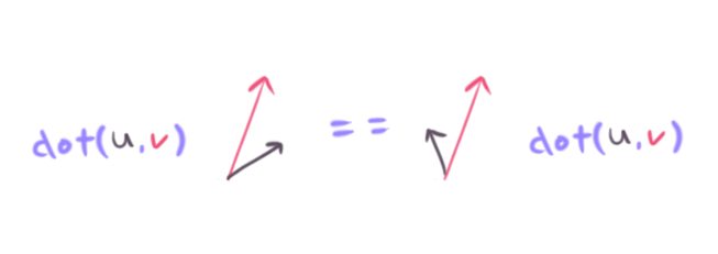
1. The dot product is commutative! dot(a, b) == dot(b, a).
2. You can algebraically manipulate scalars in and out of dot products. Example: given two vectors a and b, and a scalar s, we can see: s * dot(a, b) == dot(s * a, s * b).
3. Given two vectors u and v, if u is unit (length of 1), then dot(u, v) == the distance v travels along u.
4. If two vectors u and v are unit vectors, dot(u, v) == cos(angle between u and v).
5. Given two vectors u and v, whether or not they are unit, sign(dot(u, v)) will tell you if the vectors are facing each other or away from each other.
6. The dot product of perpendicular vectors is 0.

Point 5) begs some extra attention. The sign function means like this:

float sign(float x) { return x > 0 ? 1.0f : -1.0f; }

If the sign of dot(u, v) is positive the vectors are facing in the same direction. If dot(u, v) is negative, the vectors are facing away from each other! Therefore it’s quite useful to have a len_squared function laying around that skips the sqrtf function; if you only need to check the sign then it’s totally fine if the resulting angle is scaled.

float len_squared(v2 v) { return dot(v, v); }

Cross Product (aka 2D Determinant)

The cross product is the sibling of the dot product. It computes the sin of the angle between two vectors (scaled by the length of each vector), as opposed to the cos like the dot product. It looks quite similar, though we won’t get into the derivation for the sake of brevity. In 2D games it’s not quite as useful as the dot product, but does make its appearance occasionally. Note that the cross between two parallel vectors is 0.

My favorite example would be a function to compute the angle between two vectors. Or more specifically, the shortest angle between two vectors. Using point 5) from the last section we can write a function called shortest_arc from two vectors a and b. It returns the smallest angle needed to rotate a to b. We will name the cross product det2 for “determinant of a 2D matrix”, which will make more sense later on.

float det2(v2 a, v2 b) { return a.x * b.y - a.y * b.x; }

float shortest_arc(v2 a, v2 b)
{
	a = norm(a);
	b = norm(b);
	float c = dot(a, b);
	float s = det2(a, b);
	float theta = acosf(c);
	if (s > 0) {
		return theta;
	} else {
		return -theta;
	}
}

First we use the dot product to compute cos(theta), where theta is the angle between a and b. Unfortunately the function cos mere returns a number from -1 to 1, and that’s it. It’s just one angle. We don’t know which side of a that b points to.

In the above picture the u vector is reflected perfectly across the v vector. In both cases the dot product will return the same value, because the angle is the same in both cases! Luckily we can use det2 in a very similar way to the dot product. We can look at the sign of the cross product to see if the vector u is pointing to the left (counter-clockwise) or the right (clockwise) of the vector v. Be careful about operator order though, as det2(u, v) is not the same as det2(v, u) – in fact the sign will be flipped in these cases!

By checking the sin of det2 we know which side b is from a, wich determines the sign of the cos(theta) to resolve the mirroring issue. Please note that if you know a and b are unit vectors then the norm function calls do not need to happen. If a and b are non-unit vectors you’re likely to get a nasty NaN value from acosf.

This arc function can be used to implement all kinds of cool effects, such as an “aimer” that will track an object smoothly over time. Here’s a demonstration of tracking the mouse over time. We can call tigrMouse to get the mouse coordinate in screen space. By carefully inverting the order of operations and all the operations of world_to_screen we can implement screen_to_mouse.

v2 screen_to_world(int x, int y)
{
	v2 p = v2((float)x, (float)y);
	float half_screen_width = 640.0f / 2.0f;
	float half_screen_height = 480.0f / 2.0f;
	p.x -= half_screen_width;
	p.y -= half_screen_height;
	p.y = -p.y;
	return p;
}

v2 mouse()
{
	int x, y, buttons;
	tigrMouse(screen, &x, &y, &buttons);
	return screen_to_world(x, y);
}

#include <math.h>
#include "tigr.h"
#include "math_101.h"
#include "draw.h"

int main()
{
	screen = tigrWindow(640, 480, "Math 101", 0);

	float t = 0;
	v2 aim = v2(50, 100);
	while (!tigrClosed(screen) && !tigrKeyDown(screen, TK_ESCAPE)) {
		float dt = tigrTime();
		t += dt;
		tigrClear(screen, color_black());

		v2 m = mouse();
		draw_box(aabb(m - v2(10.0f, 10.0f), m + v2(10.0f, 10.0f)), color_white());
		float angle = shortest_arc(aim, m);
		aim = mul(sincos(angle * dt * 2.0f), aim);
		draw_vector(v2(0, 0), aim, color_white());

		tigrUpdate(screen);
	}

	tigrFree(screen);

	return 0;
}

Distance and Planes

A plane in 2D is just a line. A fancy name for a line. In 3D however, planes are like infinitely large flat sheets of paper. Another name for a plane is halfspace, because they slice all of space perfectly in half. All of these terms can be used interchangebly in 2D.

You’re probably familiar with the slope-form equation of a line.

y = mx + b

Where m is the slope factor, and b is the offset from the origin where the line crosses the y-axis. However, there’s a couple different forms of the line equation. One is called the plane equation (my favorite).

ax + by - c = 0

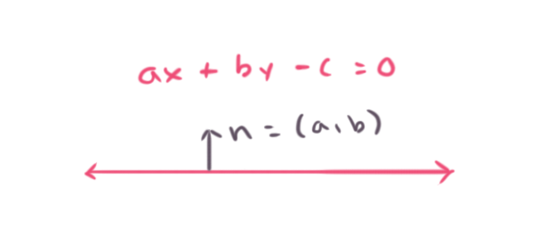
Where (a, b) is a vector called the plane normal, while (x, y) are parameters to uniquely identify any point on the plane. c is an offset from the origin, like a distance value of the plane from the origin (scaled by the length of normal (a, b)). Oftentimes the normal (a, b) is normalized to be a unit vector, this makes c the actual distance of the plane to the origin. In practice most times planes are used with unit normal vectors.

Finally there’s a parametric form which uses a single point on the line, and a vector to another point on the line.

p' = p + n * t

Where p’ is any point on the plane, p is a given point on the plane, and t is a parameter to pick a unique point on the plane. My favorite format is the plane equation ax + by - c = 0, or ax + by = c. We can make a plane type in our code, though I’d recommend calling it halfspace. Reason being: plane is often used as an identifier in other areas of the code, so we probably can avoid naming clashes by calling it a halfspace instead.

struct halfspace
{
	halfspace() { }
	halfspace(v2 n, v2 p) { this->n = n; c = dot(n, p); }
	halfspace(v2 n, float c) { this->n = n; this->c = c; }
	v2 n;
	float c;
};

Here are some extremely useful operations you can do with planes.

1. Compute the distance of a point to a plane (or just see which side of a plane a point is by looking at the sign of the distance).
2. Project a point onto the surface of a plane.
3. Compute the intersection of a line to a plane (like a raycast, more on raycasting later).

Distance Point to Plane

First up is to compute the distance of a point to a plane. Let us assume the n vector (the normal vector orthogonal to the plane’s surface, telling us which way the plane is facing) of the plane is normalized. Simply plug the point into the plane equation.

distance of point p to a halfspace (plane)
ax + by - c = 0
=>
n.x * p.x + n.y * p.y - c = distance

Note that the part n.x * p.x + n.y * p.y is a dot product. We can rewrite this as a dot product.

dot(n, p) - c = distance

And so we can write down a useful distance function for planes.

float distance(halfspace h, v2 p) { return dot(h.n, p) - h.c; }

If the distance is positive then p is on the side of the plane the normal is facing, negative otherwise.

Project Point onto Plane

Projecting a point onto a plane means moving the point to the plane’s surface by moving it the shortest distance possible. The shortest distance is along the plane’s normal vector. Therefore all we do is compute the distance to the plane, then move the point along the normal by that negated distance.

v2 project(halfspace h, v2 p) { return p - h.n * distance(h, p); }

Intersection of a Line and a Plane

This one is also quite easy if you visualize it with a drawing, but there’s also the algebraic derivation. Let’s start with the algebra. Choosing the parametric form for a line is an easy way to do it. Just note the dot product is bilinear.

line = p' = p + q * t
plane = ax + by - c = 0, or in vector form dot(n, q) - c = 0 where q is an input point

plug line equation into the plane equation
solve for t
=>
dot(n, p + q * t) - c = 0
dot(n, p) + t * dot(n, q) - c = 0
t * dot(n, q) = c - dot(n, p)
t = (c - dot(n, p)) / dot(n, q)

plug our solution for t back into the line equation to calculate p'
p' is the intersection point
=>
p' = p + q * t

v2 intersect(halfspace h, v2 p, v2 q)
{
	float t = (h.c - dot(h.n, p))) / dot(h.n, q);
	return p + q * t;
}

You’ll have trouble if the denomitator is zero (divide by zero error), which can happen if the line is parallel to the plane (recall the dot product of vectors is zero if they are perpendicular).

One thing to notice here is the numerator c - dot(n, p). This is the distance function we wrote earlier! It’s dividing the distance of the plane itself to the origin by the distance of p (the point on the line) to the origin. Recall: dotting a point with a vector gives you the distance the point travels along the vector from the origin (scaled by the vector’s length, of course).

Another way to figure out a solution is geometrically (just looking at the picture) if the line is given by two inputs points rather than parametric form (as in, the line that passes through both points).

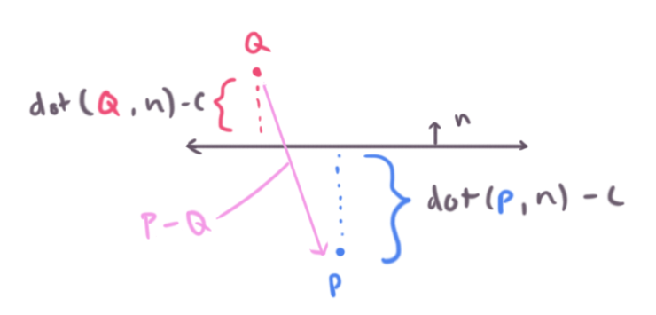
The first term dot(Q, n) - c we can call dq standing for distance of q to the plane. Similarly we have dp for distance of p to the plane.

v2 intersect(halfspace h, v2 q, v2 p)
{
	float dq = distance(h, q);
	float dp = distance(h, p);
	// ...
}

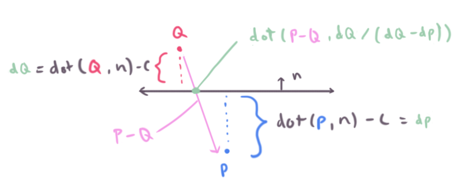
Next is to notice we can move q along the vector p - q to find the intersection point. But by how much should we move q? We know it’s some factor between the distance of p and q from the plane. Factor means a ratio or division operator. Therefore we can calculate how far along the plane’s normal p - q travels, and multiply it by this ratio to compute the intersection.

Similarly this function will fail (divide by zero) if the line is parallel to the plane, seeing the denominator for dp - dq will be zero if they are equivalent.

Another way of thinking about this is lerping from p to q. We will cover lerping more in detail later. The t value for the lerp function would be dq / (dq - dp).

v2 intersect(halfspace h, v2 q, v2 p)
{
	float dq = distance(h, q);
	float dp = distance(h, p);
	return q + (p - q) * (dq / (dq - dp));
}

Bezier Curves and Lerp

Lerp stands for linear interpolation. It means picking a number between two endpoints (a and b) based on a t value. Usually t is a value from 0 to 1. If t is 0 then you get a, otherwise if 1 you get b. Wikipedia has these three excellent images of lerping and bezier curves I’ll include below. The values of t are animating from 0 to 1, and lerp/bezier functions are used on input points p0 through p3 to move a point along a bezier curve.

float lerp(float a, float b, float t) { return a + (b - a) * t; }
v2 lerp(v2 a, v2 b, float t) { return a + (b - a) * t; }

A quadratic bezier curve is just lerping between two other lerps.

v2 bezier(v2 a, v2 b, v2 c, float t)
{
	v2 d = lerp(a, b, t);
	v2 e = lerp(b, c, t);
	return lerp(d, e, t);
}

And similarly a cubic bezier curve is just lerping between two quadratic bezier curves.

v2 bezier(v2 a, v2 b, v2 c, v2 d, float t)
{
	v2 e = bezier(a, b, c, t);
	v2 f = bezier(b, c, d, t);
	return lerp(e, f, t);
}

These are useful for animating all kinds of effects in your game, such as roller coasters, transitions from here to there, missiles, grass blowing in the wind, wires hanging from telephone poles.

As an optimization these functions can be refactored into forms where redundant calulcations are done up-front and then reused as much as possible through a bunch of fairly gnarly algebra. Let’s do it.

The first step is to unwind the lerps into their raw form.

v2 bezier(v2 a, v2 b, v2 c, float t)
{
	v2 d = lerp(a, b, t);
	v2 e = lerp(b, c, t);
	return lerp(d, e, t);
}

// -->

v2 bezier(v2 a, v2 b, v2 c, float t)
{
	v2 d = a + (b - a) * t;
	v2 e = b + (c - b) * t;
	return d + (e - d) * t;
}

Then take the algebraic pain of reducing common terms.

d = a + bt - at
e = b + ct - bt
    d + et - dt

a - at = a(1-t)
=>

d = a(1-t) + bt
e = b(1-t) + ct
    d(1-t) + et

Combine into a big formula by substituting in terms over and over
=>

   d(1-t) + et
= (a(1-t) + bt)(1-t) + (b(1-t) + ct)t

Notice that 1-t is used a lot, combine all the terms possible
=>

u = 1-t
= (au + bt)u + (bu + ct)t
= auu + but + but + ctt
= auu + but2 + ctt

v2 bezier(v2 a, v2 b, v2 c, float t)
{
	float u = 1.0f - t;
	float ut = u * t;
	v2 auu = a * u * u;
	v2 but2 = b * ut * 2.0f;
	v2 ctt = c * t * t;
	return auu + but2 + ctt;
}

And here’s a demonstration program to draw a quadratic bezier curve, and also animate a box over moving over it back and forth.

#include <math.h>
#include "tigr.h"
#include "math_101.h"
#include "draw.h"

int main()
{
	screen = tigrWindow(640, 480, "Math 101", 0);

	float t = 0;
	while (!tigrClosed(screen) && !tigrKeyDown(screen, TK_ESCAPE)) {
		float dt = tigrTime();
		t += dt;
		tigrClear(screen, color_black());

		v2 a = v2(-100, 0);
		v2 b = v2(-100, 100);
		v2 c = v2(100, 50);

		float t0 = 0;
		for (int i = 0; i <= 30; ++i) {
			float t1 = (float)i / 30.0f;
			v2 p0 = bezier(a, b, c, t0);
			v2 p1 = bezier(a, b, c, t1);
			draw_line(p0, p1, color_white());
			t0 = t1;
		}

		float pt = (cosf(t) + 1.0f) * 0.5f;
		v2 box_center = bezier(a, b, c, pt);
		draw_box(aabb(box_center - v2(10, 10), box_center + v2(10, 10)), color_white());

		tigrUpdate(screen);
	}

	tigrFree(screen);

	return 0;
}

We can also do this for the cubic bezier function. I personally do this by unwinding the calls to get all the lerps.

v2 bezier(v2 a, v2 b, v2 c, v2 d, float t)
{
	v2 e = bezier(a, b, c, t);
	v2 f = bezier(b, c, d, t);
	return lerp(e, f, t);
}

// -->

v2 bezier(v2 a, v2 b, v2 c, v2 d, float t)
{
	v2 e = lerp(a, b, t);
	v2 f = lerp(b, c, t);
	v2 g = lerp(c, d, t);
	v2 h = lerp(e, f, t);
	v2 i = lerp(f, g, t);
	return lerp(h, i, t);
}

The next step is to unwind the lerps into their raw form.

v2 bezier(v2 a, v2 b, v2 c, v2 d, float t)
{
	v2 e = a + (b - a) * t;
	v2 f = b + (c - b) * t;
	v2 g = c + (d - c) * t;
	v2 h = e + (f - e) * t;
	v2 i = f + (g - f) * t;
	return h + (i - h) * t;
}

Then take the algebraic pain of reducing common terms.

e = a + bt - at
f = b + ct - bt
g = c + dt - ct
h = e + ft - et
i = f + gt - ft
    h + it - ht

a - at = a(1-t)
=>

e = a(1-t) + bt
f = b(1-t) + ct
g = c(1-t) + dt
h = e(1-t) + ft
i = f(1-t) + gt
    h(1-t) + it

Combine into a big formula by substituting in terms over and over
=>

  h(1-t) + it
= (e(1-t) + ft)(1-t) + (f(1-t) + gt)t
= ((a(1-t) + bt)(1-t) + (b(1-t) + ct)t)(1-t) + ((b(1-t) + ct)(1-t) + (c(1-t) + dt)t)t

Notice that 1-t is used a lot, combine all the terms possible
=>

u = 1-t
= ((au + bt)u + (bu + ct)t)u + ((bu + ct)u + (cu + dt)t)t
= auuu + buut + buut + cutt + buut + cutt + cutt + dttt
= auuu + buut3 + cutt3 + dttt

v2 bezier(v2 a, v2 b, v2 c, v2 d, float t)
{
	float u = 1 - t;
	float tt = t * t;
	float uu = u * u;
	v2 auuu = a * uu * u;
	v2 buut3 = b * uu * t * 3.0f;
	v2 cutt3 = c * u * tt * 3.0f;
	v2 dttt = d * tt * t;
	return auuu + buut3 + cutt3 + dttt;
}

#include <math.h>
#include "tigr.h"
#include "math_101.h"
#include "draw.h"

int main()
{
	screen = tigrWindow(640, 480, "Math 101", 0);

	float t = 0;
	while (!tigrClosed(screen) && !tigrKeyDown(screen, TK_ESCAPE)) {
		float dt = tigrTime();
		t += dt;
		tigrClear(screen, color_black());

		v2 a = v2(-100, 0);
		v2 b = v2(-100, 100);
		v2 c = v2(100, 50);
		v2 d = v2(200, -100);

		float t0 = 0;
		for (int i = 0; i <= 30; ++i) {
			float t1 = (float)i / 30.0f;
			v2 p0 = bezier(a, b, c, d, t0);
			v2 p1 = bezier(a, b, c, d, t1);
			draw_line(p0, p1, color_white());
			t0 = t1;
		}

		float pt = (cosf(t) + 1.0f) * 0.5f;
		v2 box_center = bezier(a, b, c, d, pt);
		draw_box(aabb(box_center - v2(10, 10), box_center + v2(10, 10)), color_white());

		tigrUpdate(screen);
	}

	tigrFree(screen);

	return 0;
}

Just be careful with these optimized versions, because small values of u or t create numeric problems when multiplied together over and over. If the numbers get too small you can end up with denormalized numbers or just numerically innaccurate results. The previous version using successive lerps or more numerically stable.

Matrices

In game development matrices are mostly useful for representing transformations, namely scales, rotations and translations. In 3D graphics there’s also some projection matrices, but we’re sticking to 2D here. A matrix stores the information needed to perform a transformation upon vectors, such as placing an object into the world, or defining a relative position to another object.

Rotation Matrices

We will be using 2x2 matrices to represent rotations and scales, and later attach a position vector to create a 3x2 matrix to represent a full transform. A convenient way to look at a 2x2 matrix is like a collection of two vectors. Take a look at the matrix m.

u = (ux, uy)
v = (vx, vy)
m = [ux, vx]
    [uy, vy]

Each column of m is a vector u or v. If this matrix is a rotation matrix, then u and v would be the basis vectors. u is the x-axis and v is the y-axis. When u and v are unit vectors, and orthogonal (at 90 degree angles from each other), we call m a rotation matrix (or an orthonormal basis). We’ve actually already been using rotation matrices without knowing, back in the rotation section of this article. Let’s define our matrix struct type and a function to build a rotation matrix.

struct m2
{
	v2 x;
	v2 y;
};

m2 m2_rotation(float angle)
{
	float c = cosf(angle);
	float s = sinf(angle);
	m2 m;
	m.x = v2(c, -s);
	m.y = v2(s, c);
	return m;
}

v2 mul(m2 m, v2 v) { return v2(m.x.x * v.x + m.y.x * v.y, m.x.y * v.x + m.y.y * v.y); }

The mul function is defined by matrix multiplication rules.

If you write down the operations by hand of multiplying a rotation matrix with a vector you’ll find it to be identical to our mul function for rotations (sin + cos pair) and vectors.

               x-axis
                 v
rotation(a) = [cos(a), -sin(a)]
              [sin(a),  cos(a)]
                          ^
                        y-axis

The above matrix performs a clockwise rotation.

Matrix multiplication with vectors simply encodes a linear combination. Within that combination is our transformation (a rotation, scale, or mixture of both).

An extremely useful property of matrices is we can multiply two matrices together to concatenate their operations. If we rotate clockwise a little, then rotate counter-clockwise a lot, then multiply these together we’d be left overall with a lesser counter-clockwise rotation. We can write down the matrix mul function with our matrix to vector mul function.

m2 mul(m2 a, m2 b) { m2 c; c.x = mul(a, b.x); c.y = mul(a, b.y); return c; }

The transformation of a rotation matrix can be inverted. There actually exists an inversion operation for matrices in general, but for dimensions larger than 2x2 matrices it gets fairly expensive. A bigger problem about generic inversion functions on matrices is they encourage us to black-box matrices without knowing what the various pieces actually do or represent. For example, we know we can construct a rotation matrix out of two orthogonal unit vectors by simply placing them in the first and second columns. We already have some insight about the internals here.

We can realize quite intuitively how to invert a 2D rotation matrix without learning or bothering with a generic inversion function. We know that a 90 degree counter-clockwise rotation matrix looks like this:

[cos(a), -sin(a)]
[sin(a),  cos(a)]

If we compute the sin and cos of 90 degrees, we get these values:

[0, -1]
[1,  0]

When we multiply this matrix with a vector we can see the overall effect:

[0, -1][x]   [-y]
[1,  0][y] = [ x]

This is actually the same effect as our earlier learnings about the skew function. If we look just at the first column of our rotation matrix we can see exactly what it’s encoding when we do a multiplication with a vector. Let’s look step by step.

1.  v---------------- x * 0, The input x component will contribute 0 to the final x component.
   [0,  ][x] = [x * 0]
   [ ,  ][ ] = [  ]

2.      v------------ -1 * y, The input y component will contribute -1 to the final x component.
   [ , -1][ ] = [x * 0 + -1 * y]
   [ ,   ][y] = [  ]

   [ ,   ][x] = [x * 0 + -1 * y]
   [1,   ][ ] = [x * 1]
3.  ^---------------- 1 * x, The input x component will contribute 1 to the final y component.

   [ ,   ][x] = [x * 0 + -1 * y]
   [ ,  0][ ] = [x * 1 +  0 * y]
4.      ^----------- 0 * y, The input y component will contribute 0 to the final x component.

In steps 1-2 the linear combination for the output x-component is created. The first column in the rotatio matrix, the x-axis, decides where the new x-axis will go. A 1 in the first element means the x-axis will not change. If we move the 1 to the y-component, it means the x-axis is rotated to the y-axis. In fact, we can place any combination of -1 to 1 in the elements of the rotation matrice’s first column, so long as the columns length is 1 and the y column is orthogonal – it will be a valid rotation.

How can we perform the inverted rotation? The inverted rotation of moving the x-axis to the y-axis, would be moving the x-axis back from the y-axis.

1.
[0,  ]
[1,  ]

2.
[1,  ]
[0,  ]

3.
[ 0,  ]
[-1,  ]

4.
[-1,  ]
[ 0,  ]

Which option from 1-4 do you think might be the correct answer? Option 1 is what we already did earlier – it moved the x-axis to the y-axis, a 90 degree rotation counter-clockwise as was promised. Option 1 definitely does not invert itself. What about option 2? If we perform the math we find this means leave the x-axis unchanged. It does no operation at all. We call this an identity transform. What about options 4? This simply flips the x-axis to point backwards. That leaves option 3. It will rotate the x-axis to the y-axis but also flip it, performing a clockwise rotation. This is our 90 degree counter-clockwise rotation inverted.

Intuitively that means we can invert the y column of our rotation matrix with a negation operator as well. The full inversion of our 90-degree rotation matrix is simply to negate each element.

[ 0, 1]^-1   [0, -1]
[-1, 0]    = [1,  0]

Great! Will this work for all rotation matrices, even non-90 degree rotations? Sadly no, simple negation won’t work. However, transpose does work. Transpose simply means to make all the columns become rows, and all the rows become columns (by rotating the matrix clockwise). For any rotation it’s inverse is the transpose operation (which, for 90 degree 2D rotations is equivalent to negation).

Rotation matrix A and it's inversion B:
A^-1 = A^T = B

Here are some notable properties of rotation matrices:

1. Multiplication is non-commutative. That means A * B != B * A. If you switch around the order of operations you will get a different effect. This goes back to our old rule, listed next as number 2.
2. Rotations are always performed about the origin. Period. It’s possible to encode a larger dimensioned matrix than a mere 2x2 matrix that concatenate many rotations, translations and scales together - but each individual rotation encoded within will still have been performed about the origin. Even if the transform encodes first a translation, then a rotation, then an inverse translation (rotating about a point), the rotation itself was still done about the origin (despite it being temporarily shifted).
3. The inverse of a rotation matrix is the transposition of the rotation matrix.

Going back to m2 struct we can retrive the x-axis or y-axis of a rotation matrix any time by simply getting the x column or y column.

m2 = m2_rotation(angle);
v2 x_axis = m2.x;
v2 y_axis = m2.y;

Scale Matrices

Our 2x2 matrix, m2, can also encode a scaling factor along the x-axis or y-axis. A quick note on some properties of scale matrices.

1. They are commutative. Since a scale matrix does not rotate any axes, they act like scalar multiples. A * B = B * A.
2. The inverse of a scale operation is to divide by the same magnitude (fancy word for length/value).

The scale of our 2x2 matrices will be encoded as the length of the x-column or the y-column, representing scaling along the x-axes and y-axes respectively.

[xx, yx]
[xy, yy]

x-column/x-axis = (xx, xy)
y-column/y-axis = (yx, yy)

Scale along x-axis = |(xx, xy)|
Scale along y-axis = |(yx, yy)|

Going back to our m2 struct, we can add functionality for creating a scale matrix.

m2 m2_identity()
{
	m2 m;
	m.x = v2(1, 0);
	m.y = v2(0, 1);
	return m;
}

m2 m2_scale(float x_scale, float y_scale)
{
	m2 m = m2_identity();
	m.x *= x_scale;
	m.y *= y_scale;
	return m;
}

As hinted in the previous section on Rotation Matrices, the identity matrix is composed of a series of 1’s along the diagonal. This simply leaves each respective component unchanged during multiplication. As promised, scaling is just scaling individual axes of the matrix.

Translations

Our 2x2 m2 matrix is not designed to handle translations. However, we can augment our m2 struct by defining a wrapping struct that encompasses one more vector to store translation information. This would be a 3x2 matrix; we can call it m3x2.

struct m3x2
{
	m2 m;
	v2 p;
};

Translations don’t require too much explanation here – you’re already familiar with them! The key thing to note here is order of operations. When representing a full m3x2 matrix you can encode translations, rotations and scales all together. However, when mixing these operations you lose commutativity. Here comes another nice rule to sear into brain. Ssss…

• To undo a series of transform operations, you must not only invert each operation, but also reverse the order of operations. Example: (A * B * C)^-1 = C^-1 * B^-1 * A^-1

And finally, a function to build a translation matrix.

m3x2 make_translation(v2 p)
{
	m3x2 m;
	m.m = m2_identity();
	m.p = p;
	return m;
};

Transforms

With the nice m3x2 struct we defined in the previous section we can represent almost any kind of 2D transformation we might need, especially when we’re thinking about the three most common ones: scaling, rotating and translating.

First up, let’s list down a series of make_* functions for building our m3x2 transformation matrices, including make_translation from the previous section.

m3x2 make_identity() { m3x2 m; m.m = m2_identity; m.p = v2(0, 0); return m; }
m3x2 make_translation(v2 p) { m3x2 m; m.m = m2_identity(); m.p = p; return m; };
m3x2 make_translation(float x, float y) { return make_translation(v2(x, y)); }
m3x2 make_scale(v2 scale) { m3x2 m = make_identity(); m.x *= scale.x; m.y *= scale.y; return m; }
m3x2 make_scale(float scale_x, float scale_y) { return make_scale(v2(scale_x, scale_y)); }
m3x2 make_rotation(float radians) { m3x2 m; m.m = m2_rotation(radians); m.p = v2(0, 0); return m; }
m3x2 make_TSR(v2 p, v2 s, float radians)
{
	rotation r = sincos(radians);
	m3x2 m;
	m.x = v2(r.c, -r.s) * s.x;
	m.y = v2(r.s, r.c) * s.y;
	m.p = p;
	return m;
}

The really interesting function is make_TSR, it stands for rotate, then scale, then translate, in that order. It’s a composition of all three kinds of transformations. Whenever we multiply it with a vector, the vector will be first rotated about the origin, then scaled about the origin, then translated. Here’s the mul function for another vector.

v2 mul(m3x2 m, v2 v) { return mul(m.m, v) + m.p; }

Similarly we can follow the rules of matrix multiplication and write down how to concatenate two m3x2 matrices with a mul function.

// Transform b by a.
m3x2 mul(m3x2 a, m3x2 b) { m3x2 c; c.m = mul(a.m, b.m); c.p = mul(a.m, b.p) + a.p; return c; }

The order of operations on the translation is quite important here. We want to transform b by a, which means we want to rotate a, then scale a, then translate a. The mul with a.m does the scale/rotation together in a single m2, and the translation happens afterwards.

Transforming Objects

Usually in games you have two kinds of objects in the world: implicitly defined shapes and meshes. When I say it merely means an array of vertices. Sometimes these vertices are stored as triangle triplets, and somethings they are accompanied by an array of triangle indices. For 2D we can just stick the former: merely an array of vertices (regardless of whether they are individual points, line segments, or triangles). Think of a mesh as an array of v2’s, like the vertices of a polygon.

An implicitly defined shape reduces the amount of information needed to represent a shape down to a convenient minimum, like our aabb shape. Other common shapes include circles, capsules, and rays.

Say we have a mesh definition like so:

struct mesh
{
	array<v2> vertices;
};

Transforming this mesh with an m3x2 is an extremely common operation; simply loop over all vertices and mul them with the m3x2. This can rotate, then scale, then translate all the vertices. This is such a common thing to do that we usually attach a dedicated m3x2 onto our objects with a mesh.

struct game_object
{
	m3x2 transform;
	array<v2> mesh;
};

As a memory optimization it’s common to store a single copy of a mesh in memory, and have different objects keep a pointer to the mesh and a transform. The mesh vertices themselves, as they sit in memory, are usually stoerd in what’s called model space. This just means the vertices are likely very close to the origin and haven’t been rotated/scaled/translated into the world yet.

To draw one of the meshes usually the vertices are copied over to the GPU (graphics processing unit). In tigr we just set pixels onto the screen directly. Whenever we want to draw a mesh we can loop over the vertices, mul them in the loop and use temporary v2 variables to represent the transformed verts. Then we draw with those temporary variables. The original source mesh vertices are as if they are in “read-only mode”.

struct game_object
{
	m3x2 transform;
	array<v2>* mesh;
};

// This is just example code -- with tigr we aren't sending meshes to the GPU. But, for most games
// this is an extremely common operation. We just use tigr for a nice and simple learning environment.
void send_triangle_mesh_to_gpu(game_object* o)
{
	v2* vertices = o->mesh.data();
	int size = o->mesh.size();
	m3x2 m = o->m;
	for (int i = 0; i < size; I += 3) {
		v2 a = vertices[i];
		v2 b = vertices[i + 1];
		v2 c = vertices[i + 2];
		a = mul(m, a);
		b = mul(m, b);
		c = mul(m, c);
		gpu_context->add_triangle(a, b, c);
	}
}

For an implicitly defined shape we can do the same, but scaling might be a bit difficult. For example how can we scale a circle along the x-axis but not the y-axis? It’s a bit of a condundrum on what to do here. Nonetheless we can make a decision.

struct circle
{
	v2 p;
	float r;
};

circle mul(m3x2 m, circle c)
{
	c.r *= len(m.x);
	c.p = mul(m, c.p);
	return c;
}

In the above example we chose to use the x-axis for scaling circles. How you decide to handle this case in your game is up to you. You could use the y-axis, you could use the min or max of both axes, or even the average of both axes.

Object Heirarchies

It’s quite common to give your game_object (or equivalence) a transform and a parent. The parent would be a reference, pointer or id to a parenting game object. The parent has it’s own transform, while the game_object would have it’s transform be defined relative to the parent’s transform. If a game object has no parent, it’s transform is absolute, and not relative.

This can be useful to compose more complicated looking game objects. A great example would be 2D games that use skeletal animation for the animations. Each “bone” in a skeleton is merely a transformation matrix (like an m3x2). An image or mesh is placed into each bone, which each bone transformed relative to it’s parent. A good way to learn about what skeletal animations look like is to check out these cool live demos by Spine software. Some examples of games that use skeletal animation would be:

• Plants vs Zombies
• Slay the Spire

Raycasting Basics

A ray is a like a line. It starts at a point and goes on infinitely in a direction. However for games actual rays aren’t super useful because they usually cause a performance concern. When we test to see if a ray hits anything, if the ray goes on infinitely it will often query against shapes in the world very far away that aren’t relevant. Instead it’s good design to define a ray for our games as a line-segment with a finite length.

struct ray
{
	v2 p;    // Start position.
	v2 d;    // Direction of the ray (normalized)
	float t; // Distance along d the ray travels.
	v2 endpoint() { return p + d * t; }
};

It’s quite important to keep the ray direction normalized for numeric stability during ray test operations. Here’s a thread talking about this sort of thing in detail.

The equation for a ray is merely the parametric form of a line with a condition attached.

p is the start point of the ray
d is the ray direction vector (normalized)
x is an input scalar

p' = p + d * x
x >= 0

In our code we apply an extra condition, namely that the ray goes from t = 0 to t = N. So we can rewrite the definition more like this.

p' = p + d * x
x >= 0
x <= t // t comes from our ray struct, defining the endpoint of the ray's line segment

We can cast rays and hit-test all kinds of shapes. We will cover some shapes here:

1. Ray to circle
2. Ray to polygon

Ray to Circle

Deriving the ray to circle routine is much like our other exercises: write down some equations and plug them into each other.

q : input point
c : center of circle
t : distance along the ray that might hit the circle

sqrt((q - c)(q - c)) = r
p + d * t

rewrite circle equation
=>
|q - c|^2 = r^2

substitute ray into q
=>
|p + d * t - c|^2 = r^2

solve for t (time of impact)
(p + d * t - c)(p + d * t - c) - r^2 = 0
((p - c) + t * d)((p - c) + t * d) - r^2 = 0
e = p - c
(e + t * d)(e + t * d) - r^2 = 0
dot(e, e) + t * dot(e, d) + t * dot(e, d) + t^2 * dot(d, d) - r^2 = 0
t^2 * dot(d, d) + 2t * dot(e, d) + dot(e, e) - r^2 = 0

quadratic equation in t
t = (-b ± sqrt(b * b - 4ac))/(2a)
a = dot(d, d)
b = 2 * dot(d, e)
c = dot(e, e) - r^2

The discriminant (part in the sqrt) tells information based on the sign.
If it's positive we have an intersection.

bool raycast_circle(ray r, circle c)
{
	v2 c = b.c;
	v2 p = a.p;
	v2 e = p - c;
	v2 d = a.d;
	float a = dot(d, d);
	float b = 2.0f * dot(e, d);
	float c = dot(e, e);
	float t = a.t;
	float rr = b.r * b.r;
	float discriminant = b * b - 4.0f * a * c;
	return discriminant > 0;
}

The first obvious optimization is that we know d to be of unit length, so dot(d, d) is 1.

bool raycast_circle(ray r, circle c)
{
	v2 p = a.p;
	v2 e = p - c.p;
	v2 d = a.d;
	float rr = b.r * b.r;
	float b = 2.0f * dot(e, d);
	float c = dot(e, e) - rr;
	float discriminant = b * b - 4.0f * c;
	return discriminant > 0;
}

Another thing is to use a different form of the quadratic equation where b is doubled. This can remove the extra constant multiply by four and by two. This also slightly increases numeric stability by keeping the numbers a little lower.

t^2 * dot(d, d) + 2t * dot(e, d) + dot(e, e) - r^2 = 0
t = (-b ± sqrt(b * b - ac))/a
a = 1
b = dot(d, e)
c = dot(e, e) - r^2

bool raycast_circle(ray r, circle c)
{
	v2 p = a.p;
	v2 e = p - c.p;
	v2 d = a.d;
	float rr = b.r * b.r;
	float b = dot(e, d);
	float c = dot(e, e) - rr;
	float discriminant = b * b - c;
	return discriminant > 0;
}

Lastly, it’s generally useful to add the hit point and normal to the output of any raycast function. The normal describes the direction the surface is facing where the ray hit. This can be used to inform where bullets should bounce, or how players are standing on top of objects. Simply solving for t and plugging it into the ray equation p + d * t will give us the hit location. But first, we must make sure t is within the bounds of the line segment. If t is negative it means the ray started inside the sphere. Additionally, we ignore the ± and only consider the earliest hit time, which would be the - case in our quadratic solution t = -b - sqrt(b * b - c).

struct raycast_output
{
	float t; // Time of impact.
	v2 n;    // Normal of the surface at impact (unit length).
};

struct ray
{
	ray() { }
	ray(v2 p, v2 d, float t) { this->p = p; this->d = d; this->t = t; }
	v2 p;    // Start position.
	v2 d;    // Direction of the ray (normalized)
	float t; // Distance along d the ray travels.
	v2 endpoint() { return p + d * t; }
	v2 impact(raycast_output hit_data) { return p + d * hit_data.t; }
};

// Reflect vector d across vector n. See: http://paulbourke.net/geometry/reflected/
v2 reflect(v2 d, v2 n) { return d - n * 2 * dot(d, n); }

bool raycast_circle(ray r, circle c, raycast* out)
{
	v2 e = a.p - c.p;
	float rr = b.r * b.r;
	float b = dot(e, a.d);
	float c = dot(e, e) - rr;
	float discriminant = b * b - c;
	bool missed_circle = discriminant < 0;
	if (missed_circle) return false;
	t = -b - sqrtf(discriminant);
	if (t >= 0 && t <= r.t) {
		out->t = t;
		v2 impact = r.p + r.d * t;
		out->n = norm(impact - c.p);
	} else {
		return 0;
	}
}

Here’s main.cpp for the above demo.

#include "tigr.h"
#include "math_101.h"
#include "draw.h"

circle circles[] = {
	circle(-100, 0, 20),
	circle(-200, 50, 30),
	circle(-150, 150, 70),
	circle(50, 200, 100),
	circle(200, -150, 70),
	circle(0, -100, 20),
	circle(-150, -200, 100),
};

void cast_ray(ray r, int depth = 0, int depth_max = 100)
{
	if (depth == depth_max) {
		draw_vector(r.p, r.endpoint() - r.p, color_white());
	}
	float min_t = FLT_MAX;
	raycast_output best_hit;
	for (int i = 0; i < sizeof(circles) / sizeof(*circles); ++i) {
		raycast_output hit_data;
		bool hit = raycast(r, circles[i], &hit_data);
		if (hit && depth < depth_max) {
			if (hit_data.t < min_t) {
				min_t = hit_data.t;
				best_hit = hit_data;
			}
		}
	}
	if (min_t != FLT_MAX) {
		v2 hit = r.impact(best_hit);
		draw_line(r.p, hit, color_white());
		r.d = reflect(r.d, best_hit.n);
		r.p = hit;
		r.t -= best_hit.t;
		cast_ray(r, depth + 1, depth_max);
	} else {
		draw_vector(r.p, r.endpoint() - r.p, color_white());
	}
}

int main()
{
	screen = tigrWindow(640, 480, "Math 101", 0);

	float t = 0;
	while (!tigrClosed(screen) && !tigrKeyDown(screen, TK_ESCAPE)) {
		float dt = tigrTime();
		t += dt;
		tigrClear(screen, color_black());

		for (int i = 0; i < sizeof(circles) / sizeof(*circles); ++i) {
			draw_circle(circles[i], color_white());
		}

		v2 m = mouse();
		ray r = ray(v2(0, 0), norm(m), 25.0f + (cosf(t * 2.0f) + 1.0f) * 0.5f * 500.0f);
		cast_ray(r);

		tigrUpdate(screen);
	}

	tigrFree(screen);

	return 0;
}

Ray to Polygon

We’ve actually covered this topic already back in the Distance and Planes section, at least, mostly covered it by calculating distances of points to planes, and intersection of line segment to plane. From Christer Ericson’s excellent book Real-Time Collision Detection he explains a great algorithm for raycasting against a polygon.

Ericson describes the process as continually slicing a line segment with cutting planes, where each plane is a face of the polygon. If the ray is completely sliced away (length becomes 0 or negative) there is no intersection. Otherwise the final line segment contains the start/endpoints for the ray intersections. Special care must be taken to avoid dividing by zero. The image below shows the step-by-step process of clipping a ling segment against invidual planes of a polygon.

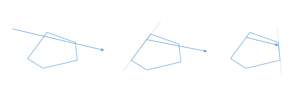
The code is rather straightforward. Compute the numerator and denominator in our earlier discussions of line segment to plane, avoid divide by zero issues, and keep track of a lo/hi time of intersection. Just be sure that the polygon is in counter-clockwise vertex order, and is a valid convex hull. We’ll go over an algorithm for building 2D convex hulls later. Note we can of course use this algorithm on aabb’s as well (though it wouldn’t quite be optimal, will definitely get the job done and likely be more than fast enough for most games).

#define POLYGON_MAX_VERTS 8

struct polygon
{
	int count = 0;
	v2 verts[POLYGON_MAX_VERTS];
	v2 norms[POLYGON_MAX_VERTS];
	void compute_norms()
	{
		for (int i = 0; i < count; ++i) {
			int j = i + 1 < count ? i + 1 : 0;
			norms[i] = norm(skew(verts[i] - verts[j]));
		}
	}
};

bool raycast(ray r, polygon poly, raycast_output* out)
{
	float lo = 0;
	float hi = r.t;
	int index = ~0;

	for (int i = 0; i < poly.count; ++i) {
		// Calculate distance of point to plane.
		// This is a slight variation of dot(n, p) - c, where instead of pre-computing c as scalar,
		// we form a vector pointing from the ray's start point to a point on the plane. This is
		// functionally equivalent to dot(n, p) - c, but we don't have to store c inside of our poly.
		float distance = dot(poly.norms[i], poly.verts[i] - r.p);
		float denominator = dot(poly.norms[i], r.d);
		if (denominator == 0) {
			// Ray direction is parallel to this poly's face plane.
			// If the ray's start direction is outside the plane we know there's no intersection.
			if (distance > 0) return false;
		} else {
			float t = distance / denominator;
			if (denominator < 0) {
				// Ray is entering the plane.
				lo = max(lo, t);
				index = i;
			}
			else hi = min(hi, t); // Ray is exiting the plane.
			bool ray_clipped_away = lo > hi;
			if (ray_clipped_away) return false;
		}
	}

	if (index != ~0) {
		out->t = lo;
		out->n = poly.norms[index];
		return true;
	} else {
		return false;
	}
}

You might be wondering why the polygon is limited to merely 8 vertices with POLYGON_MAX_VERTS. It’s possible to change this to some other value, such as 16 or 32, but in practice it’s often not a very useful thing to do. In 2D if there are too many vertices the shape starts to look a lot less unique, more like a circle or ellipse. It’s very convenient to keep implementations extremely simple by limiting the number of vertices to a small number. This makes polygons memcpy-able, and very cache-friendly for running quick and efficient code.

Collision Detection Basics

Detecting collisions between shapes is quite a difficult challenge. It takes a lot of diligence to learn all the mathematics covered in this article up to this point. We will cover a couple select algorithms to get you started, but a full discussion of collision algorithms is a bit out of scope. Some additional resources are linked at the end of this section.

Implicit Shapes

Implicitly defined shapes are ones we can represent with a small bit of information, as opposed to storing a mesh or array of vertices. Good candidates in 2D include circles, capsules, rays, and axis aligned boxes (aabb). Here’s my recommendation on how to setup your implicit shapes to make writing collision detection routines as easy as possible. Note these definitions were all provided earlier in this document (they’re the same as before).

struct circle
{
	circle() { }
	circle(v2 p, float r) { this->p = p; this->r = r; }
	circle(float x, float y, float r) { this->p = v2(x, y); this->r = r; }
	v2 p;
	float r;
};

#define POLYGON_MAX_VERTS 8

struct polygon
{
	int count = 0;
	v2 verts[POLYGON_MAX_VERTS];
	v2 norms[POLYGON_MAX_VERTS];
	void compute_norms()
	{
		for (int i = 0; i < count; ++i) {
			int j = i + 1 < count ? i + 1 : 0;
			norms[i] = norm(skew(verts[i] - verts[j]));
		}
	}
};

struct aabb
{
	aabb() { }
	aabb(v2 min, v2 max) { this->min = min; this->max = max; }
	v2 min;
	v2 max;
};

struct raycast_output
{
	float t; // Time of impact.
	v2 n;    // Normal of the surface at impact (unit length).
};

struct ray
{
	ray() { }
	ray(v2 p, v2 d, float t) { this->p = p; this->d = d; this->t = t; }
	v2 p;    // Start position.
	v2 d;    // Direction of the ray (normalized)
	float t; // Distance along d the ray travels.
	v2 endpoint() { return p + d * t; }
	v2 impact(raycast_output hit_data) { return p + d * hit_data.t; }
};

Circle to Circle

Once we compute the distance between two circle centers, using the Pythagorean Theorem, we can compare it to the sum of the radii. If the radii are longer than the distance the circles interesect, otherwise they don’t intersect.

bool circle_to_circle(circle circ_a, circle circ_b)
{
	v2 d = circ_b.p - circ_a.p;
	float d2 = dot(d, d);
	float r = circ_a.r + circ_b.r;
	return d2 < r * r;
}

In order to resolve this collision a bit more information is needed such as the depth of the collision, and a vector to push the shapes away from each other. The best vector would be the axis of minimum penetration. It means the axis with the smallest signed distance to separate the shapes. You can find more information about this special axis by reading online about the Separating Axis Test.

For the case of circles the axis is always going to be the normalized vector from one circle center to another, except when the circles are perfectly on top of each other, where we must choose an arbitrary axis to push along.

Collision Manifold

The information gathered from a collision routine on how shapes are touching is often called the collision manifold. It’s a fancy word that means the topology (surface) of an enclosed shape (convex shapes in our case). Often times this manifold information will be used for one of two major purposes:

1. Physics engines to resolve collisions semi-realistically.
2. Gameplay logic to understand how things hit each other, like what the surface is like when a player walks upon it.

The manifold should consist of penetration depth (how deeply shapes are intersecting), a collision normal (the axis of minimum penetration), and optionally points of contact along the collision plane. Here’s an example struct definition:

struct collision_data
{
	int count;
	v2 points[2];
	float depth[2];
	v2 normal;
};

For more advanced collision routines a time of impact may also be calculated and represented as a single float t from 0 to 1.

The reason points is an array of up to two unique points is that the collision manifold exists within the contact plane. This means the plane orthogonal to the axis of minimum separation. The 2D cross-section of a convex polygon is merely a line segment, so two points suffices. In 3D however, more points are needed. Depending on the physics engine it could be anywhere from 3-8 points in practice, 4-5 being a golden spot. These hit points are mostly needed for phyics engines. If gameplay is the only customer then a single point of contact is likely all that’s necessary, if any at all.

We can augment our circle collision function to generate a manifold in the event a collision is detected. For now I will generate a single contact point for simplicity. By convention we can name each input shape a and b respectively, and always generate a hit_spot on the surface of b.

struct collision_data
{
	bool hit = false;
	v2 hit_spot;
	float depth;
	v2 normal;
};

collision_data circle_to_circle(circle circ_a, circle circ_b)
{
	collision_data out;
	v2 d = circ_b.p - circ_a.p;
	float d2 = dot(d, d);
	float r = circ_a.r + circ_b.r;
	if (d2 < r * r) {
		out.hit = true;
		out.hit_spot = circ_b.p - norm(d) * circ_b.r;
		out.depth = r - len(d);
		out.normal = norm(d);
	}
	return out;
}

This function still suffers from numeric robustness problems. If circles a and b are right on top of each other the length of d will be 0 and cause norm to fail with a division by zero error. In the case of zero distance we can simply choose an arbitrary axis for n. This also lends itself to a minor optimization where len is only called once (as we omit the extra calls to norm that call len internally).

collision_data circle_to_circle(circle circ_a, circle circ_b)
{
	collision_data out;
	v2 d = circ_b.p - circ_a.p;
	float d2 = dot(d, d);
	float r = circ_a.r + circ_b.r;
	if (d2 < r * r) {
		float l = len(d);
		d = l == 0 ? v2(0, 1) : d * (1.0f / l);
		out.hit = true;
		out.hit_spot = circ_b.p - d * circ_b.r;
		out.depth = r - l;
		out.normal = d;
	}
	return out;
}

As you can see, generating the manifold requires a lot of extra work and implementation! But the information is very valuable for physics and gameplay alike.

AABB to AABB

Here’s the typical aabb to aabb test. It simply checks the four face planes by looking directly at the x and y components of min and max elements of our aabb struct.

bool aabb_to_aabb(aabb a, aabb b)
{
	if (b.max.x < a.min.x) return false;
	if (a.max.x < b.min.x) return false;
	if (b.max.y < a.min.y) return false;
	if (a.max.y < b.min.y) return false;
	return true;
}

This function can be optimized to remove excess branching so the branch predictor cannot fail.

bool aabb_to_aabb(aabb a, aabb b)
{
	bool d0 = b.max.x < a.min.x;
	bool d1 = a.max.x < b.min.x;
	bool d2 = b.max.y < a.min.y;
	bool d3 = a.max.y < b.min.y;
	return !(d0 | d1 | d2 | d3);
}

You may be wondering why we used bitwise or | instead of conditional or ||. The conditional operator will often generate branches in assembly structure, as defined by the C standard if the first of a conditional fails the rest need not be checked. By using the bitwise operator we instead perform four bitwise or’s without any branching logic at all. This makes our function run in constant and predictable time with no branching.

As usual, generate a mafifold is way harder than merely detecting a collision. The algorithm works by checking for overlap on first the x-axis and then the y-axis. This is very similar to the previous test, but actually calculates an overlap distance rather than just checking for a sign with the < operator. If either axis is separating we can immediately return no interesction (due to the Separating Axis Test).

Otherwise we must see if the boxes are intersecting more on the x or y-axis. Once known we can immediately deduce a good contact point and the surface normal.

collision_data aabb_to_aabb(aabb a, aabb b)
{
	collision_data out;
	v2 mid_a = (a.min + a.max) * 0.5f;
	v2 mid_b = (b.min + b.max) * 0.5f;
	v2 ea = abs((a.max - a.min) * 0.5f);
	v2 eb = abs((b.max - b.min) * 0.5f);
	v2 d = mid_b - mid_a;

	// calc overlap on x and y axes
	float dx = ea.x + eb.x - abs(d.x);
	if (dx < 0) return out;
	float dy = ea.y + eb.y - abs(d.y);
	if (dy < 0) return out;

	v2 n;
	float depth;
	v2 p;

	if (dx < dy) {
		// x axis overlap is smaller
		depth = dx;
		if (d.x < 0) {
			n = v2(-1.0f, 0);
			p = mid_a - v2(ea.x, 0);
		} else {
			n = v2(1.0f, 0);
			p = mid_a + v2(ea.x, 0);
		}
	}  else {
		// y axis overlap is smaller
		depth = dy;
		if (d.y < 0) {
			n = v2(0, -1.0f);
			p = mid_a - v2(0, ea.y);
		} else {
			n = v2(0, 1.0f);
			p = mid_a + v2(0, ea.y);
		}
	}

	out.hit = true;
	out.hit_spot = p;
	out.depth = depth;
	out.normal = n;
	return out;
}

Circle to AABB

The circle to aabb collision detection function is a lot like the circle to circle collision detection function. The trick is to compute the closest point on the aabb to the circle, then perform a circle to circle test with a radius of 0. In older literature the closest point is often called L, so we copy that old naming convention here for fun. But if I were you I’d probably name it “closest_point”.

float clamp(float v, float lo, float hi) { return min(max(v, lo), hi); }
v2 clamp(v2 v, v2 lo, v2 hi) { return v2(clamp(v.x, lo.x, hi.x), clamp(v.y, lo.y, hi.y)); }

bool circle_to_aabb(circle a, aabb b)
{
	v2 L = clamp(a.p, b.min, b.max);
	v2 ab = a.p - L;
	float d2 = dot(ab, ab);
	float r2 = a.r * a.r;
	return d2 < r2;
}

You guessed it – writing the manifold version is way harder. We start off the same, calculating L the closest point on the box to the circle. There are two cases to look for: shallow and deep intersections. If the circle center intersects the box it’s a deep interesction, shallow otherwise.

For the shallow case we simply treat the problem as two circles, where the circle on L has a radius of 0. For the deep case we snap the sphere’s center to the box’s exterior, immediately giving us all our manifold pieces (the normal, the depth and a collision point on the surface of the aabb).

collision_data circle_to_aabb(circle a, aabb b)
{
	collision_data out;
	v2 L = clamp(a.p, b.min, b.max);
	v2 ab = a.p - L;
	float d2 = dot(ab, ab);
	float r2 = a.r * a.r;

	if (d2 < r2) {
		if (d2 != 0) {
			// shallow (center of circle not inside of AABB)
			float d = sqrtf(d2);
			v2 n = norm(ab);
			out.hit = true;
			out.depth = a.r - d;
			out.hit_spot = a.p + n * d;
			out.normal = n;
		} else {
			// deep (center of circle inside of AABB)
			// clamp circle's center to edge of AABB, then form the manifold
			v2 mid = (b.min + b.max) * 0.5f;
			v2 e = (b.max - b.min) * 0.5f;
			v2 d = a.p - mid;
			v2 abs_d = abs(d);

			float x_overlap = e.x - abs_d.x;
			float y_overlap = e.y - abs_d.y;

			float depth;
			v2 n;

			if (x_overlap < y_overlap) {
				depth = x_overlap;
				n = v2(1.0f, 0);
				n *= (d.x < 0 ? 1.0f : -1.0f);
			} else {
				depth = y_overlap;
				n = v2(0, 1.0f);
				n *= (d.y < 0 ? 1.0f : -1.0f);
			}

			out.hit = true;
			out.depth = a.r + depth;
			out.hit_spot = a.p - n * depth;
			out.normal = n;
		}
	}

	return out;
}

Convex Hull

Computing the convex hull from a set of points is a critical operation for collision detection. In 2D usually hulls are defined by a set of counter-clockwise vertices. The convexity of a convex hull allows us to perform a variety of very useful collision detection tests without too much trouble.

This mainly comes from the planes of the convex hull. Each plane of a convex hull corresponds to one of the faces. If we visualize the negative space behind a plane as the half of all space pointing away from the plane’s normal vector, we notice for a convex hull the interior is te negative space. Another way to rephrase this: inside the convex hull is behind all of the face planes.

Point in Polygon (Convex)

A similar observation pops up for the outside of a convex hull – outside of a convex hull is on the positive space of at least one of the planes. This lets us write down a very simple and efficient routine to detect point in convex polygon.

bool point_in_poly(polygon poly, v2 p)
{
	for (int i = 0; i < poly.count; ++i) {
		float c = dot(poly.norms[i], poly.verts[i]);
		float dist = dot(poly.norms[i], p) - c;
		if (dist >= 0) return false;
	}
	return true;
}

Other Convex Hull Tests

Here are some other particularly interesting tests you can consider learning about outside of this article. This article is already too long, so I can’t cram in all these details in one place!

• Point in concave polygon (ray odd/even hit test), Ericson Real-Time Collision Detection
• Polygon to Polygon via SAT (separating axis theorem/test)
• Broadphase, or Bounding Volume Heirarchy (BVH) (especially the dynamic aabb tree by E. Catto)
• Time of impact (TOI), swept collision detection, or continuous collision

Computing a Convex Hull

From reading Christer Ericson’s orange book Real-Time Collision Detection we can implement the simplest algorithm I know of for computing a 2D convex hull, Andrew’s algorithm. The only predicate used is the det2 function to figure out if a set of vertices are on counter-clockwise or clockwise order. The main step of the algorithm looks at three points and forms two vectors each starting from one point, and pointing to the other two points. This is exactly like our section on the shortest_arc function using the det2 function. Here is the algorithm:

1. First sort all the input points from smallest to largest on the x-axis. To break ties, sort from smallest to largest on the y-axis.
2. Add the two left-most vertices to the hull. The first will be on the convex hull, while the second is tentative.
3. Check the next vertex, going from left to right, and see if it’s on the left (counter-clockwise negative) or right (clockwise positive) using det2.
4. If the vertex is more left than our tentative vertex, pop the tentative vertex off the hull and and replace it with the next vertex.
5. Continue steps 3-4 until we reach a tentative vertex that creates a clockwise orientation, or run out of points to pop.
6. Complete once we loop over all the points. We have added the top-half or bottom-half of the hull (depending on how you compute the inputs to det2, in our example below this was the bottom-half).
7. Repeat the process for the other half of the hull.
8. Remove the extra point at the end of the hull output.

Check out this animation of the algorithm from wikibooks on Andrew’s Algorithm.

// Andrew's Algorithm from Ericson's Real-Time Collision Detection book.
int convex_hull(v2* verts, int count)
{
	count = min(count, POLYGON_MAX_VERTS);
	if (count < 3) {
		return 0;
	}

	// Sort lexicographically (on x-axis, then y-axis).
	for (int i = 0; i < count; ++i) {
		int lo = i;
		for (int j = i+1; j < count; ++j) {
			if (verts[j].x < verts[lo].x) {
				lo = j;
			} else if (verts[j].x == verts[lo].x && verts[j].y < verts[lo].y) {
				lo = j;
			}
		}
		v2 swap = verts[i];
		verts[i] = verts[lo];
		verts[lo] = swap;
	}

	int j = 2;
	int hull[POLYGON_MAX_VERTS + 1];
	hull[0] = 0;
	hull[1] = 1;

	// Find lower-half of hull.
	for (int i = 2; i < count; ++i) {
		while (j >= 2) {
			v2 e0 = verts[hull[j-1]] - verts[hull[j-2]];
			v2 e1 = verts[i] - verts[hull[j-2]];
			if (det2(e0, e1) <= 0) --j;
			else break;
		}
		hull[j++] = i;
	}

	// Find top-half of hull.
	for (int i = count-2, k = j+1; i >= 0; --i) {
		while (j >= k) {
			v2 e0 = verts[hull[j-1]] - verts[hull[j-2]];
			v2 e1 = verts[i] - verts[hull[j-2]];
			if (det2(e0, e1) <= 0) --j;
			else break;
		}
		hull[j++] = i;
	}

	--j; // Pop the last vert off as it's a duplicate.
	if (j < 3) return 0;
	v2 hull_verts[POLYGON_MAX_VERTS];
	for (int i = 0; i < j; ++i) hull_verts[i] = verts[hull[i]];
	memcpy(verts, hull_verts, sizeof(v2) * j);
	return j;
}

Slicing a Convex Hull

Sutherland-Hodgman clipping algorithm for Dynamic Shape Slicing (an article I wrote some time ago) is a great way to make use of convex hulls. Rather than get into all the details I’ll just recommend you check out my other article if you’re interested! Here’s the source code for the function to split a polygon in into front and back polygons along a splitting plane split.

struct sutherland_hodgman_output
{
	polygon front;
	polygon back;
};

bool in_front(float distance, float epsilon) { return distance > epsilon; }
bool behind(float distance, float epsilon) { return distance < -epsilon; }
bool on(float distance, float epsilon) { return !in_front(distance, epsilon) && !behind(distance, epsilon); }

// See: https://gamedevelopment.tutsplus.com/tutorials/how-to-dynamically-slice-a-convex-shape--gamedev-14479
sutherland_hodgman_output sutherland_hodgman(halfspace split, polygon in, const float k_epsilon = 1.e-4f)
{
	sutherland_hodgman_output out;
	v2 a = in.verts[in.count - 1];
	float da = distance(split, a);

	for(int i = 0; i < in.count; ++i) {
		v2 b = in.verts[i];
		float db = distance(split, b);

		if(in_front(db, k_epsilon)) {
			if(behind(da, k_epsilon)) {
				v2 i = intersect(b, a, db, da);
				out.front.verts[out.front.count++] = i;
				out.back.verts[out.back.count++] = i;
			}
			out.front.verts[out.front.count++] = b;
		} else if(behind(db, k_epsilon)) {
			if(in_front(da, k_epsilon)) {
				v2 i = intersect(a, b, da, db);
				out.front.verts[out.front.count++] = i;
				out.back.verts[out.back.count++] = i;
			} else if(on(da, k_epsilon)) {
				out.back.verts[out.back.count++] = a;
			}
			out.back.verts[out.back.count++] = b;
		} else {
			out.front.verts[out.front.count++] = b;
			if(on(da, k_epsilon)) {
				out.back.verts[out.back.count++] = b;
			}
		}

		a = b;
		da = db;
	}

	return out;
}

Advanced Collision Detection

More advanced collision detection routines are out of scope for this article. Things like Capsule and Polygon collisions require quite lot of complicated mathematics and code. That’s all for another time and another blog post! For now you can find a full implementation of correctly implemented and efficient 2D collisions routines at cute_c2.h, a small single-file C library. It covers circles, capsules, polygons, aabbs, rays, convex hull, shape expansion, closest point pairs, and time of impact (swept) collision detection.

Toy Demo

THIS POST IS A WIP