Deriving OBB to OBB Intersection and Manifold Generation
The Oriented Bounding Box (OBB) is commonly used all over the place in terms of simulation and game logic. Although often times OBBs aren’t actually bounding anything, and really just represent an implicitly defined box.
OBBs commonly come in 2D and 3D form, though there aren’t all that many resources on the internet describing how to derive the 3D case. The ability to write robust collision detection, and more importantly manifold generation (contact data needed to resolve the collision), relies on a good understanding of linear algebra and geometry.
Readers will need to know about affine and linear transformations, and have intuition about the dot and cross products. To learn these preliminaries I highly recommend the book “Essential Mathematics” by Jim Van Verth. I will also be assuming readers are familiar with the Separating Axis Theorem (SAT). If you aren’t familiar with SAT please do a short preliminary research on this topic.
The fastest test I’m aware of for detection collision between two OBBs, in either 2 or 3 dimensions, makes use of the Separating Axis Theorem. In both cases it is beneficial to transform one OBB into the space of the other in order to simplify particular calculations.
Usually an OBB can be defined something like this in C++:
// Example of a 3D OBB
struct OBB
{
  Mat3 r; // world space x, y and z axes (local axes of this OBB)
  Vec3 c; // center of the OBB
  Vec3 e; // half widths along x, y and z axes
};
6 Face Axes
As with collision detection against two AABBs, OBBs have x y and z axes that correspond to three different potential axes of separation. Since an OBB has local oriented axes they will most of the time not line up with the standard Euclidean basis. To simplify the problem of projecting OBB A onto the the axes of OBB B, all computations ought to be done within the space of A. This is just a convention, and the entire derivation could have been done in the space of B, or even in world space (world space would have more complex, and slow, computations).
The translation vector t is defined as:

Where C_i denotes the center of an OBB (it means C subscript i, like in the above image), and R denotes the rotation of an OBB. t points from A’s center to B’s center, within the space of A. The relative rotation matrix to transform from B’s frame to A’s frame is defined as:

C can be used to transform B’s local axes into the frame of A. In A’s own frame it’s local axes line up with the standard Euclidean basis, and can be directly computed with the half width extents e_a.
To calculate the separation s along the local axis l from an OBB examine the following diagram and matching equation:
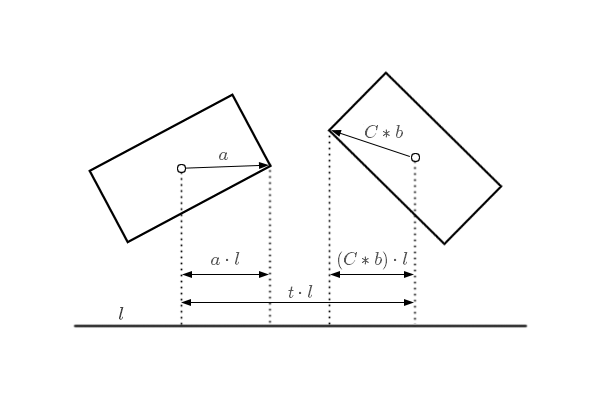

Due to symmetry the absolute value of a projection can be used in order to gather a value that can be used to represent a projection along a given direction. In our case we aren’t really interested in the sign of the projection and always want the projection towards the other OBB. I understand that newer programmers may have some trouble translating math into code, so here’s an example of eq 1) as C++:
// Using the OBB definition from earlier in this post
float s = dot(t, l) - (A.e.x + dot(abs(C).column0(), B.e));
s is the separation along an axis. t is the translation vector from center of one box to another. l is the axis we are projecting onto (in this case A’s x axis).
9 Edge Axes
In 2D eq 1) is all that is needed to detect overlap upon any given possible axis of separation. In 3D a new topological feature arises on the surface of geometry: edges. Because edges form entirely separate Voronoi regions from face surfaces they can also provide possible axes of separation. With OBBs it is fast to test all possible unique edge axes of separation.
Given two edges upon two OBBs in 3D space the vector perpendicular to both would be the possible axis of separation, and can be computed with a cross product. A possible 9 axes of separation arise from crossing each local axis of A with the each local axis of B.
Since C is composed of a concatenation between (R_a)^T and R_b, the rows of this matrix can be thought of as the local axes of B in the space of A. When a cross product between two axes is required to test separation, the axis can be pulled directly out of C. This is much faster than computing a cross product in world space between two arbitrary axis vectors.
Lets derive a cross product between A’s x axis and B’s z axis, all within the space of A. In A’s space A’s x axis is:

In A’s space B’s z axis is:

The axis l is just the cross product of these two axes. Since A’s x axis is composed largely of the number 0 elements of C can be used to directly create the result of the cross product, without actually running a cross product function. We arrive to the conclusion that for our current case:

This particular l axis can be used in eq 1) to solve for overlap.
Since the matrix C is used to derive cross product results the sign of the elements will be dependent on the orientation of the two OBBs. Additionally, the cross product will negate on of the terms in the final axis. Since eq 1) requires only absolute values it may be a good idea to precompute abs(C), which takes the absolute value element by element. This computation can be interleaved between the different axis checks for the first 6 checks, only computed as needed. This may let an early out prevent needless computation.
The same idea can be used to derive this axis in the space of B by crossing B’s local z axis with A’s local x axis transformed to the space of B. To do this it may be easy to use C^T, which represents:

More information about this can be found in my previous article about the properties of transposing a matrix concatenation.
Eventually all axes can be derived on paper and translated into code.
Manifold Generation
A collision manifold would be a small bit of information about the nature of a collision. This information is usually used to resolve the collision during physical simulation. Once an axis of least penetration is found the manifold must be generated.
For SAT manifold generation is quite straight forward. The entirety of the details are expressed very well by Dirk Gregorius’ great online tutorial from GDC 2013. The slides are openly available for free, and currently hosted here by Erin Catto. Readers are encouraged to familiarize themselves with the idea of reference and incident faces, as well as the idea of reference face side planes.
There are only two different cases of collision that should be handled: edge to edge and something to face. Vertex to edge, vertex to face, and vertex to vertex resolutions are ill-defined. On top of this numerical imprecision makes detecting such cases difficult. It makes more sense in every way to skip these three cases and stick to the original two.
Something to Face
Something has hit the face of one of the OBBs. It can be anywhere from 1 to 4 vertices from the face of the opposing OBB. The entire intersecting volume between two OBBs does not need to be considered due to the nature of SAT and the axis of minimum penetration. Only two faces from each OBB need be considered for this case, and are by convention named the reference and incident faces, one from each OBB.
Finding the incident face given an axis of separation can be found in constant time with implicit geometry like an OBB; the problem reduces to that of finding a vector that most faces a given vector, or in other words the most negative dot product.
Once the incident face is identified it is clipped to the side planes of the reference face. There may be some tricks involving basis transformations here to simplify the clipping routine. In order to perform clipping the incident face vertices must be calculated. Given a face normal from an OBB all four face vertices can be computed with the normal and the half width extents of the OBB. In similar fashion the side planes of the reference face can also be directly computed.
Edge to Edge The edge to edge case requires a clever constant-time computation of a supporting edge. A supporting edge is the edge most pointed to by a given axis of separation. The computation of this edge may be tricky to derive yourself, though there do exist online references. I suggest checking out Open Dynamics Engine (ODE) by Russell Smith, or the Cyclone Engine by Ian Millington for information on how to compute a supporting edge.
Once both supporting edges are calculated the closest two points between each edge can be calculated and used as a single contact point of which to resolve upon.
Numeric Stability
In all uses of OBB to OBB intersection cross products with nearly parallel vectors pose a problem. The best solution is to detect when any two axes from each OBB are parallel and skip all nine cross product axes. It can be visually shown that no false positives will come from skipping the cross product axes in this case.
A simpler solution, as proposed by Gottschalk ’00 in his paper “Collision Queries using Oriented Bounding Boxes”, which made its way into Ericson’s book “Real-Time Collision Detection”, is to bias all elements of C with a small epsilon to drive near-zero axes away from a degenerate case. For other axes the epsilon value should be tuned such that it doesn’t have much an impact upon results.
If using this collision routine to resolve collision during physical simulation certain tuning my be appropriate. If an iterative resolver is used it may be preferred to have slightly more consistent manifold generation, as opposed to exact manifold generation. For details I suggest researching works by Erin Catto and comments made by others around the Bullet Forums.
AABB to OBB
Hopefully by now readers realize that this whole time we’ve been simplifying the problem of OBB to OBB to the problem of AABB to OBB. When an actual AABB needs to be collided against an OBB simplifications can occur. Many simplifications revolve around the non-necessity to transform things into the basis of the AABB, since world coordinates should suffice.
One Axis Aligned (or Two?)
Some games have OBBs that only orient on some of their axes instead of all of them. One can immediately realize that no cross product checks need to be performed in any case, if two OBBs have orientation locked on the same axis. Other optimizations will occur as well, making some axis tests reduced to that of AABB overlap testing.
Conclusion
Collision detection is difficult. Writing robust collision detection code requires a good mathematical foundation as well as the ability to write efficient code. This slight mixture of fields of study may be difficult to learn all at once, but it all gets easier with time and practice and the rewards can be very fulfilling.
I’d like to thank my friend Nathan Carlson for teaching much of this information to me, and for his insightful discussions.
Here is a finished implementation: link to github.